-
Pleistocene Coastal Plain sand dunes and the value of pattern recognition in LiDAR interpretation
by Philip S. Prince
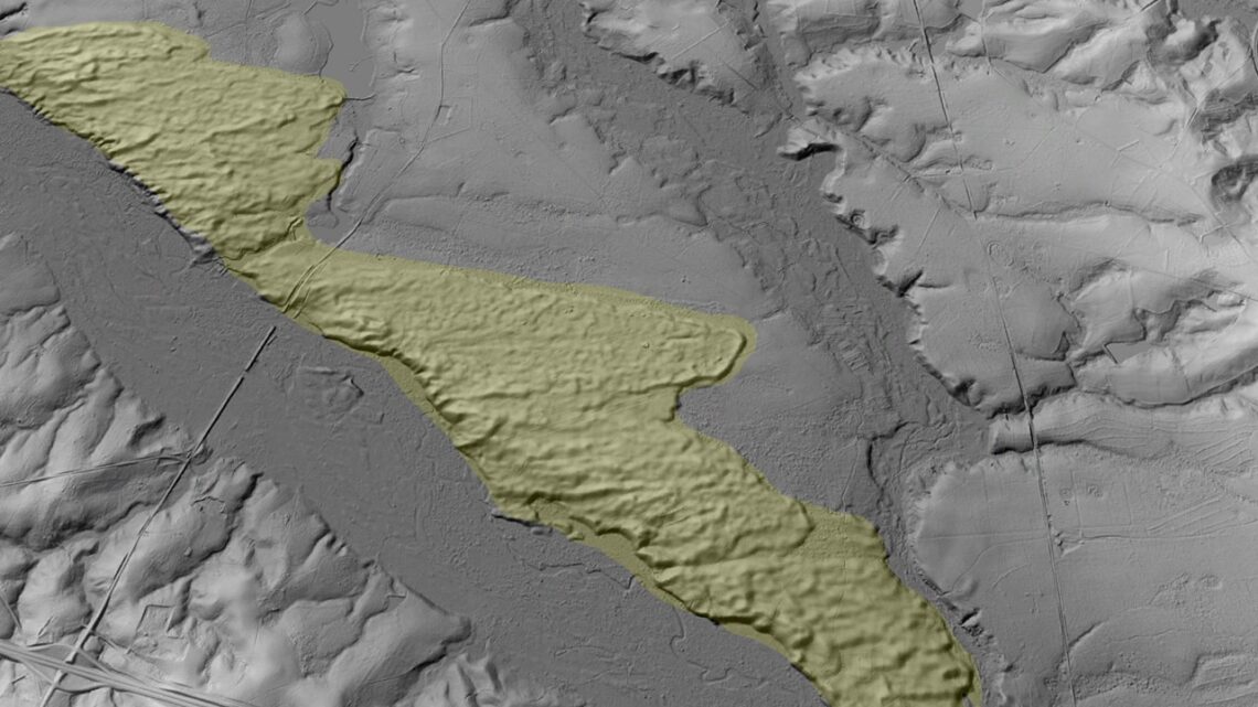
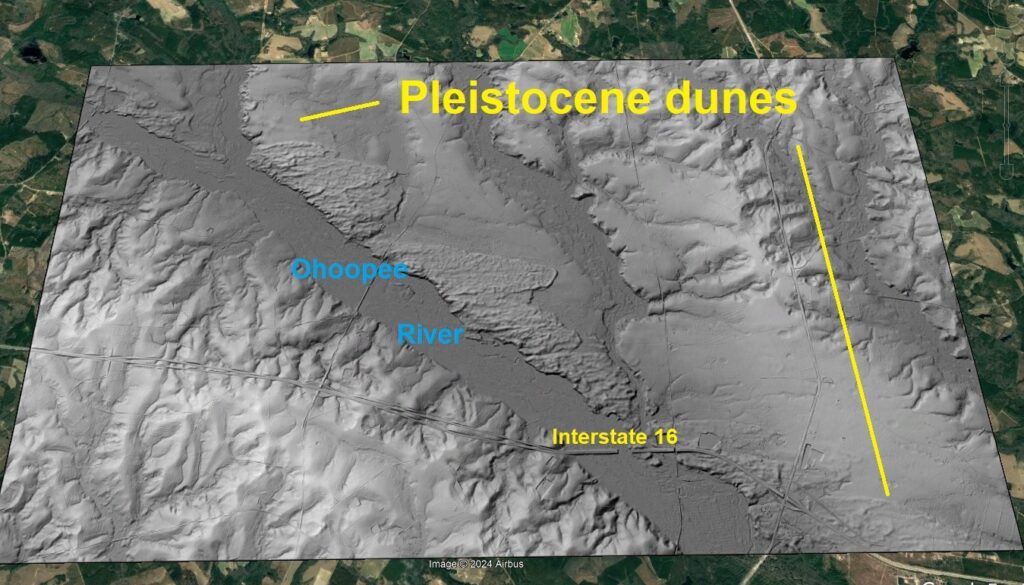
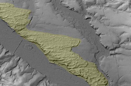
Pleistocene-aged sand dunes are some of the most conspicuous lidar features of the southeastern United States Coastal Plain, largely because their lumpy surfaces and non-erosional outlines contrast sharply with other “background” landforms. It’s hard to imagine the modern-day swampy Coastal Plain being much less forested and windy enough to be covered with migrating sand dunes, but high-resolution lidar imagery shows just how widespread these features once were. A particularly beautiful set of dunes is visible with lidar imagery on the east bank of the Ohoopee River west of Metter, Georgia, just north of Interstate 16.
Wind direction was from left to right (west to east), and the sand in the dunes was derived from sandy coastal plain sediments exposed in the bluff carved by the Ohoopee River. Dunes like these are interesting landforms to examine with lidar because their shape implies the material movement that formed them–it’s easy enough to imagine wind sweeping the sand across the landscape. An intersting detail of these ancient dunes is how their sandy soil controls agriculture. Note how the bright, sandy soil is visible in places where farmed trees have been harvested in the image above. I’m not exactly sure why, but tree farming closely follows the boundaries of the old dunes very closely, as seen below.
Looking for features like these dunes is a good way to train for pattern recognition in lidar evaluation, as the dunes are not as conspicuous when the observer is “zoomed out.” Once identified, however, the dunes are quite distinct from background erosional features (stream channels, etc.) and are consistent in their appearance within the region.
Interpreting landforms like the dunes with lidar imagery also requires understanding of modern-day, active features whose origin and evolution is known. There are plenty of modern dune features to see in Google Earth, and (unsurprisingly) they bear a striking resemblance to the Pleistocene Ohoopee dunes. The dunes shown below are a nice example; they have developed above a river bluff in northern Alaska.
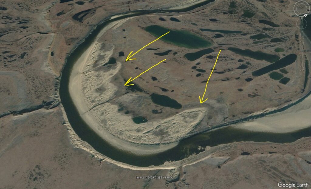
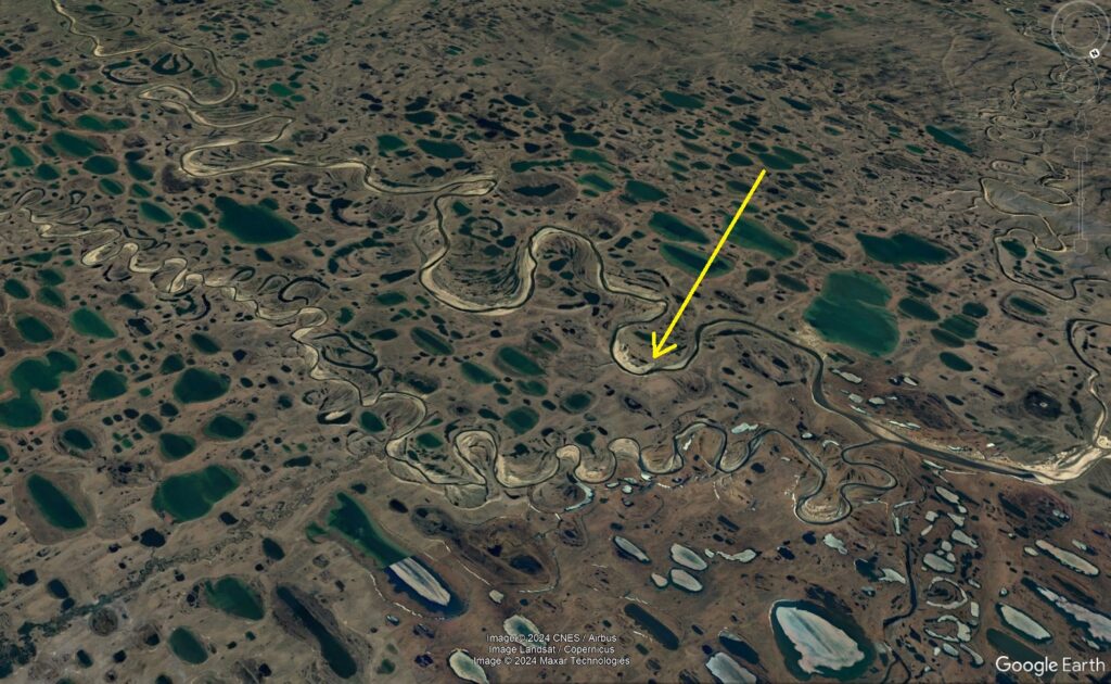
Interestingly, modern-day northern Alaska has been suggested as a good indicator of what the Pleistocene Coastal Plain landscape was like. These Alaska dunes are located in a landscape full of elliptical, wind-sculpted lakes that are a dead ringer for Carolina Bays as well. Carolina Bays and modern-day landscape comparisons need their own post, but the similarities between these Alaskan features and many aspects of the southern Coastal Plain landscape are almost uncanny. In the image below, the yellow arrow points to the river bluff dunes shown above. The swarms of elliptical lakes are obvious enough. Lakes near the lower right edge of the image are partially covered in ice.
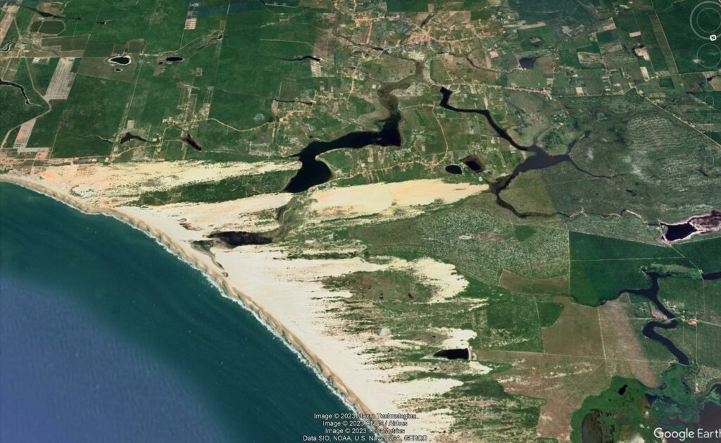
Dune development is a product of the laws of physics and the materials involved, not latitude or geography, and good examples along topographic bluffs can be found throughout the modern world. The coast of central Brazil has some outstanding dune fields that are useful in identifying and interpreting old, vegetated features like the Ohoopee dunes.
The island of K’gari in Queensland, Australia, is another good example.
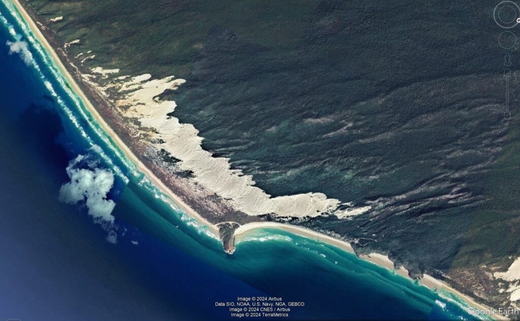
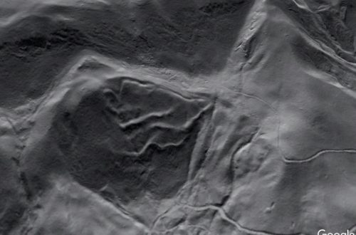
The consistency of dune shape between all of these locations is a nice example of patterns and their recognition in the Earth system. By thinking about landforms as expressions of a given process, anyone interested in geology can work logically towards understanding why a particular location looks like it does. Pattern recognition is a good way to link the study of older, sometimes partially preserved landforms with the modern landscape to allow accurate interpretation of features that might otherwise be mystifying. After looking at the images in this post, some landforms in the lidar image below might be more recognizable.
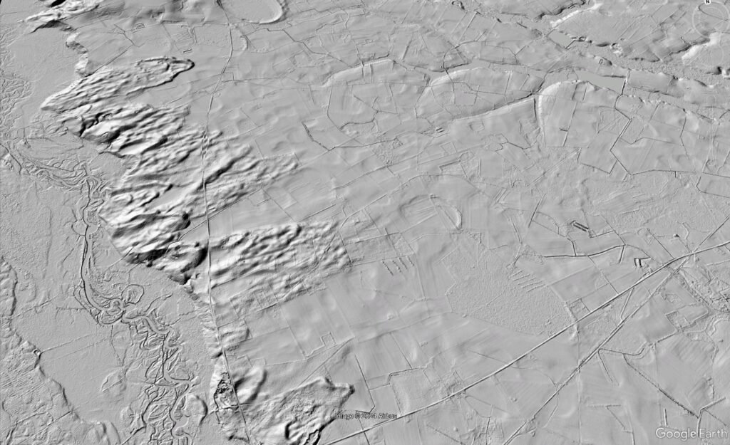
This image is from Lee County, South Carolina, just north of Lee State Park. The Lynches River (left side of the image) carved bluffs into sandy Coastal Plain sediments, which provided a sand source for Pleistocene winds. These dune features are analogous to the Ohoopee River dunes, which are quite far away but located in a comparable geologic setting under the same Pleistocene climate regime. An observer need not be an expert in South Carolina geology to interpret this lidar image; understanding material movement and dune development in the Earth system is far more useful.
A closer look at the Lee County image reveals hundreds of small, elliptical, and very faint “pock marks,” with a few larger ones mixed in. These are Carolina Bays, which remain “officially” unexplained. Take a look back at the second Alaska image and see what you think in terms of pattern recognition…
-
Lidar highlights impressive landslide density on the southern Appalachian Blue Ridge Escarpment, western North Carolina
by Philip S. Prince
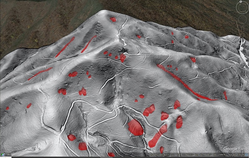
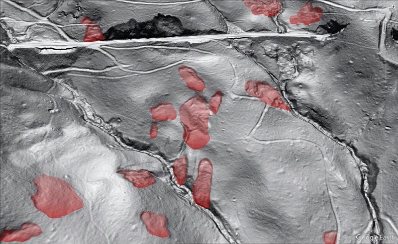
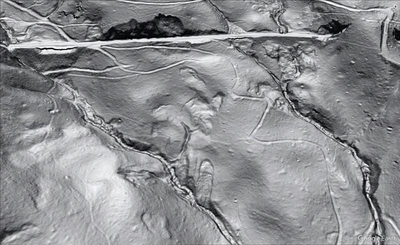
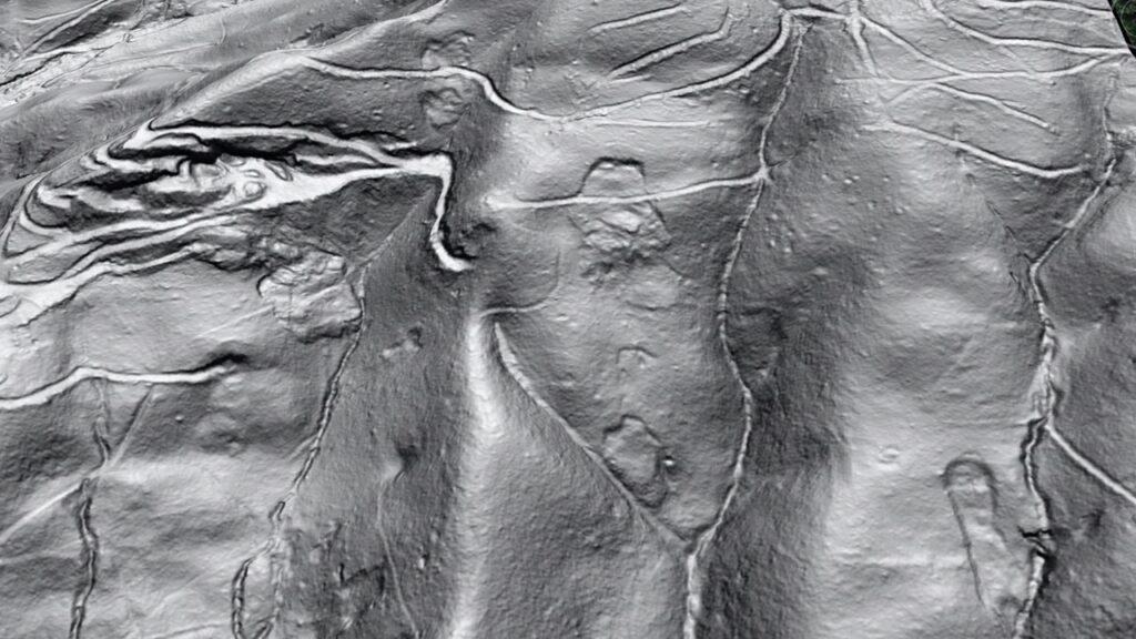
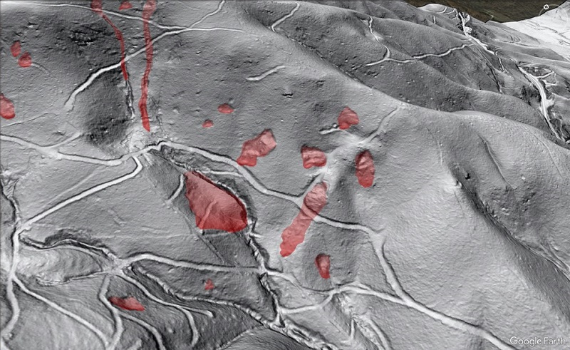
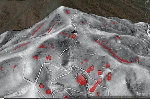
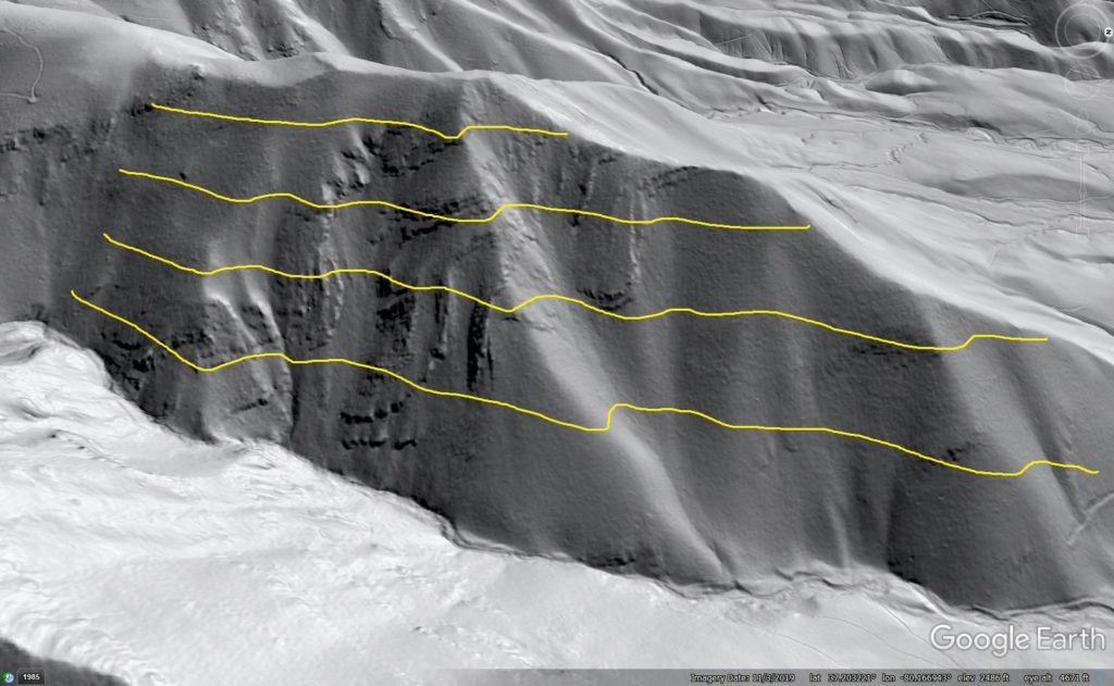
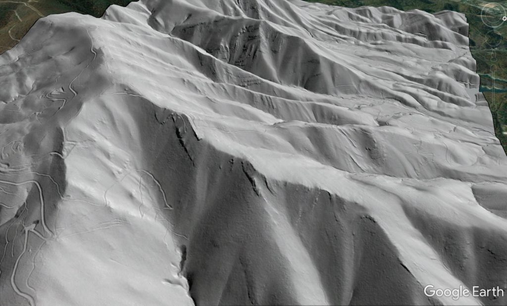
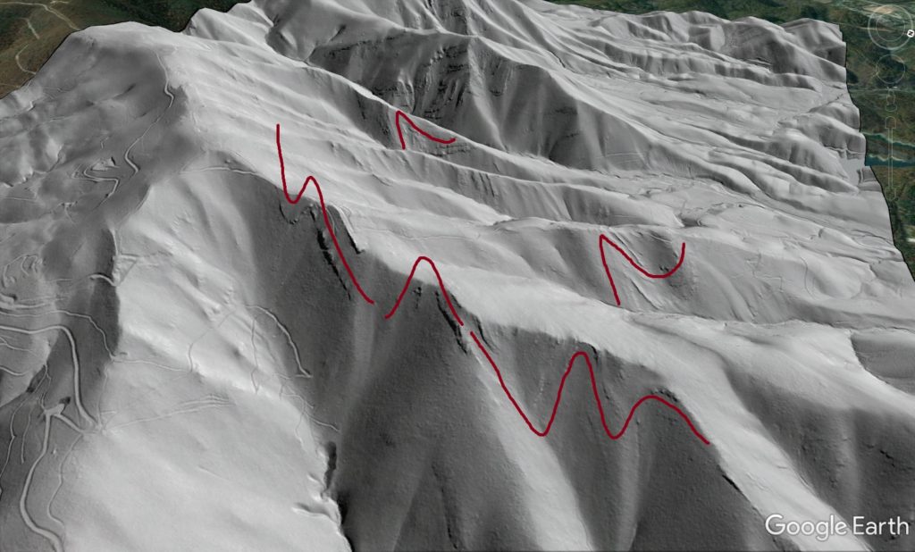
Landslides occur regularly along the rugged Blue Ridge Escarpment in western North Carolina, and lidar imagery provides a way to easily view the accumulated scars of these events that are preserved in the landscape. With a high quality (0.5-meter resolution) lidar dataset, it’s hard to examine much of the Escarpment without seeing a few landslide features. Some slopes have more than others, however, and I think the McDowell County slope shown below probably has the greatest density of slides I have seen in the last 3 years of mapping. The transparent red areas cover definite (or very high confidence) slide features. The yellow arrow points to an active railroad line to provide a sense of scale…possible slides on railroad cut slopes or embankments are not marked.
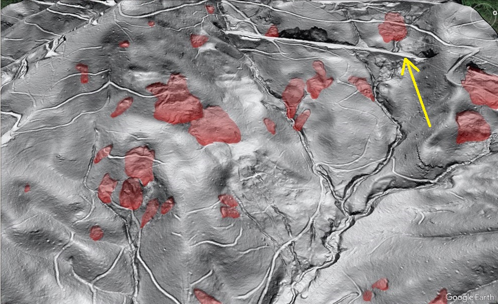
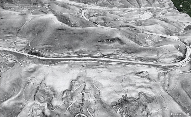
The area shown above is surprisingly small to host so many slides. The area with marked slides covers about 0.3 square miles, or 0.8 square kilometers (204 acres or 85 hectares); this excludes the distant slopes seen at upper left, where no slides are marked. Like so much of Appalachia, the slides are not visible without lidar imagery. Despite their crisp outlines, many are cut by undamaged logging road grades, suggesting the slides are many decades old. The GIF below compares aerial imagery, unmarked lidar slopeshade, and marked lidar slopeshade.
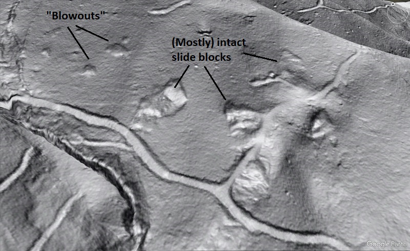
Many of the slides occur in clusters and are not significantly displaced. The cluster of slides above right center and below the railroad grade is worth a look in detail.
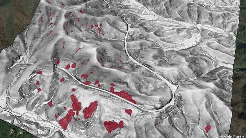
The images shown above are captured from kmz files I made, and a zoomed-out view provides some larger scale context. The previous images are from area A1.
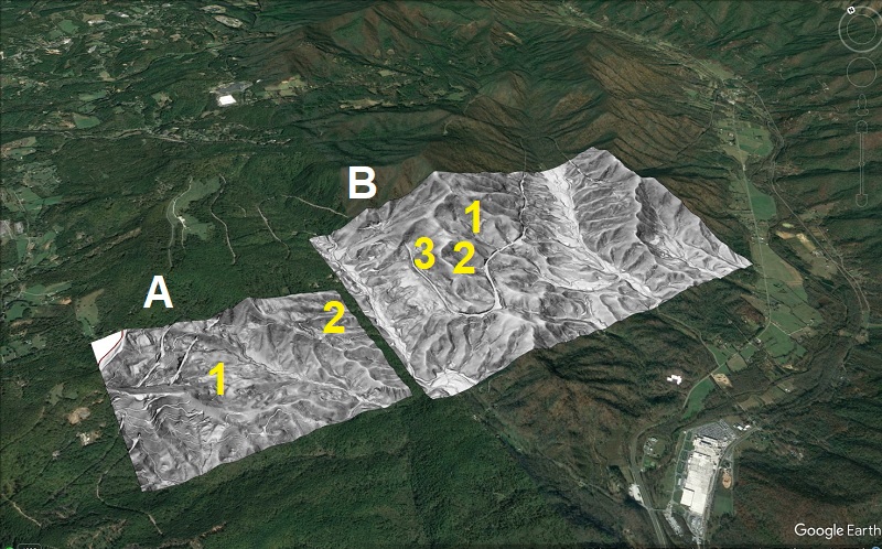
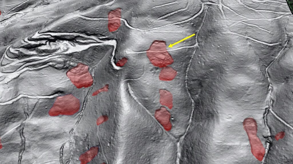
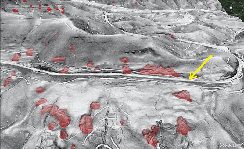
Area A2 shows comparable slide density, with numerous minimally displaced, largely intact slides. The slide indicated by the yellow arrow is 130 ft (40 m) across. The road grades are single-track logging roads. Notably, they are not offset by the upper two slides…this is more clear in the lower, unmarked image.
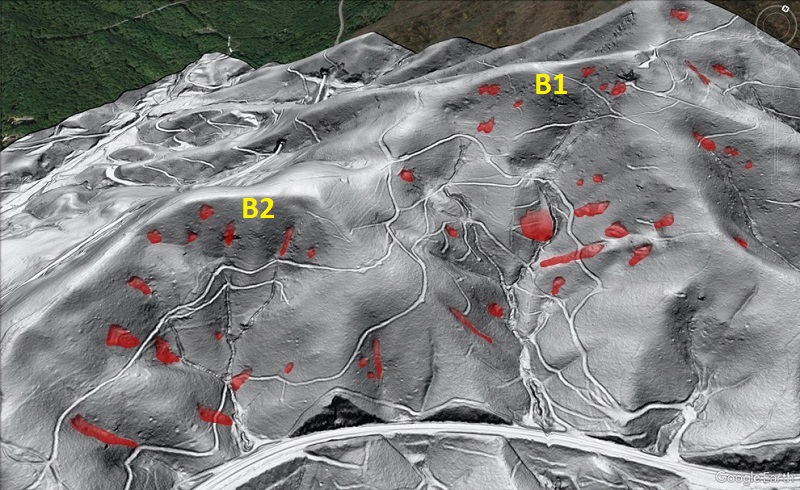
Similar landslide density is visible in area B1. The style of the slides is somewhat different–many are small “blowout”-type slides. This difference in style may result from the different aspect of the slope with respect to underlying bedrock structures.
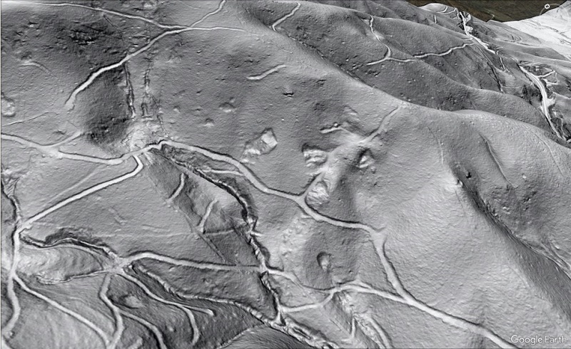
The central portion of the image above provides a nice view of the contrast in slide style and the resulting traces in the landscape.
Both areas B1 and B2 host a very high number of slides. Again, the railroad grade at the base of the image provides some sense of scale. None of the slides marked in the image below are seen to offset any of the logging road grades, despite the crisp, well-defined appearance of the slides.
Area B3, just over the ridge (to the left) of B2 above, is also a mess. The arrow points to the railroad line for reference.
Area B3 is distinct in terms of its aspect and its relationship to bedrock structure. Dip of bedrock foliation at B3 is significantly less steep than the slopes above the railroad line, creating cliffs and ledges. Lidar imagery suggests that large amounts of colluvium and talus have accumulated below these ledges. Failure in colluvial deposits is widespread in the region, particularly as the deposits weather, so a slope like this is certainly expected to show evidence of failure, regardless of land use or construction.
An overall view looking north across area B shows slide distribution across the face of the Escarpment towards the valley at upper right. This isn’t a perfect labeling of each and every slide, but it’s pretty good. Slide density does decline significantly below the railroad grade and is much less on the distant ridge at top and right.
So, why have so many landslides occurred on these slopes? The most likely explanation is an extreme precipitation event. This area was heavily impacted in both 1916 and 1940 by extreme rainfall events, and the clustering of slides and their lack of damage to mid-20th century road grades would fit a connection to either of the storms nicely. These McDowell County slopes also resemble slopes in the headwaters of the Moorman’s River west of Charlottesville, Virginia, which experienced numerous slides due to an exceptional thunderstorm event in 1995. The two Moorman’s River slopes shown below (in lidar hillshade instead of slopeshade) reveal numerous slides that cluster in a similar fashion to the McDowell County examples. As usual, single-track logging roads provide a sense of scale.
Details of bedrock geology, colluvial or residual soil development, shallow groundwater, and land use may also control the McDowell County slide clusters. Because of the area’s history of extreme rainfall events and land use, many variables may have worked together to produce the high density of landslides. They may not have occurred together, either, although their comparable preservation and pre-logging road development suggests that they could have. This area will received detailed landslide mapping in the coming months, and field investigation may shed more light into the details of the slides’ setting. Until then, just knowing what the land surface looks like and what sort of slope behavior is possible in the area is useful and interesting.
-
Erosion and scour in sandbox model debris flows (microbeads and cohesive substrate)
by Philip S. Prince
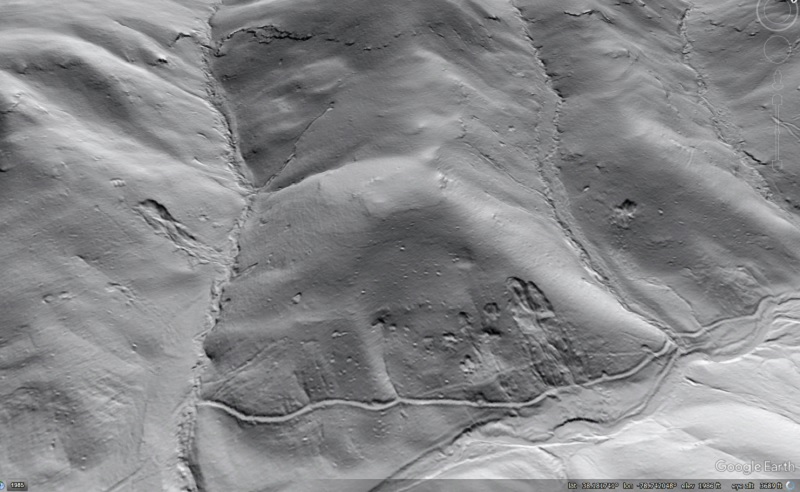
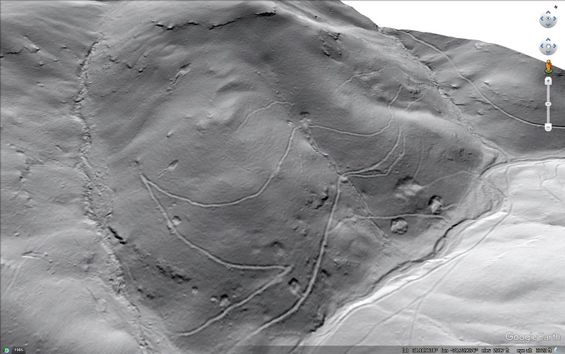
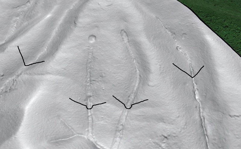
The speed and mobility of debris flows make them particularly dangerous among landslides. Debris flows move so quickly because they are fluidized masses of saturated soil, boulders and rock fragments, wood, and water, which causes them to erode or scour their flow path and accumulate more material than initially failed on the slope. The eroded track left by the scouring process is often clearly visible in lidar imagery, as in the case of the two debris flows shown below. These flows occurred in July 1995 near Buena Vista, Virginia, in the Appalachian blue Ridge. The respectively round and elliptical failed areas, along with the scoured tracks, stand out in comparison to “normal” ravines and channels on the slope.
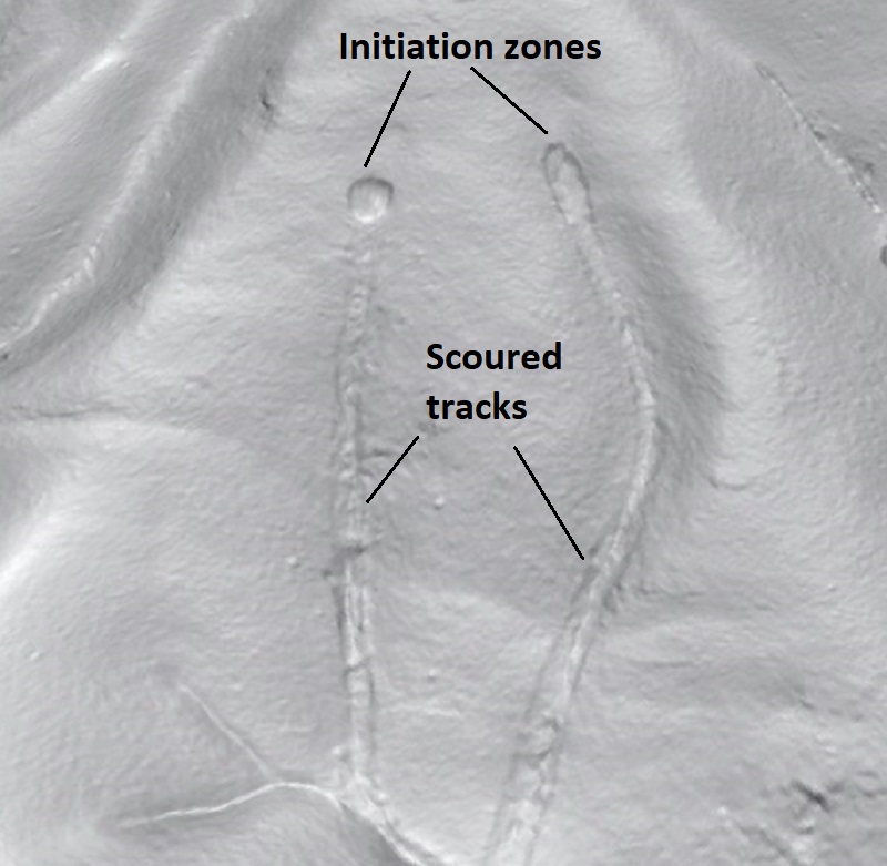
The failure scars (at the head of the scoured tracks) are about 65 ft (20 m) wide. The flows were about 25 years old when this Google Earth imagery was taken, and forest recovery in the scoured tracks is still limited to hardy species like pines. Looking more closely at the scoured tracks, they show a U-shaped profile compared to the typical V-shaped profile of channels or ravines sculpted by water alone.
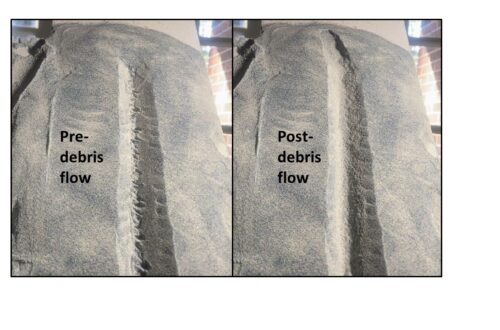
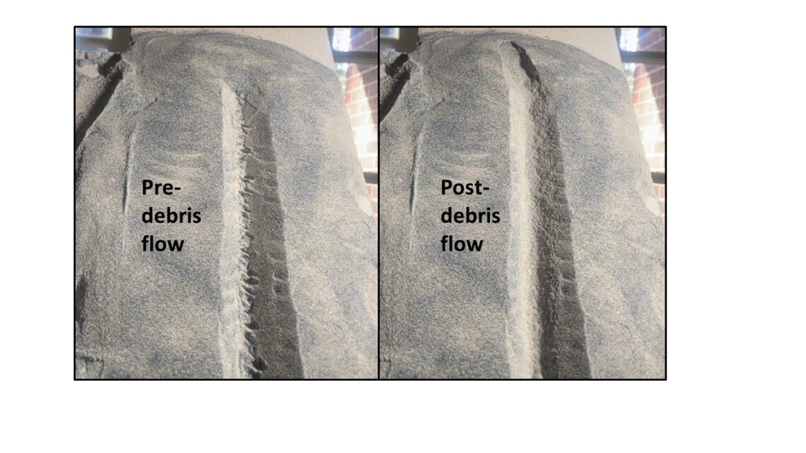
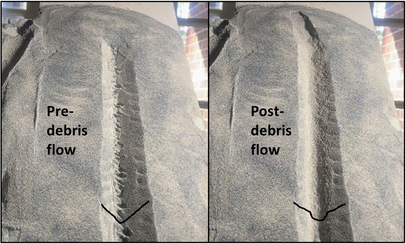
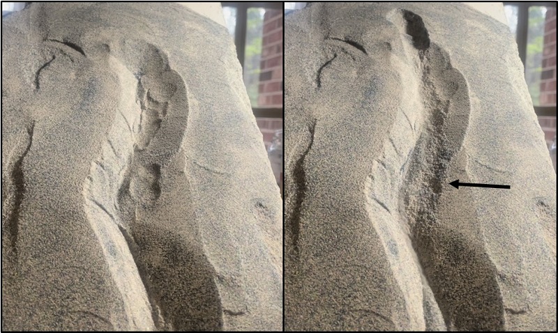
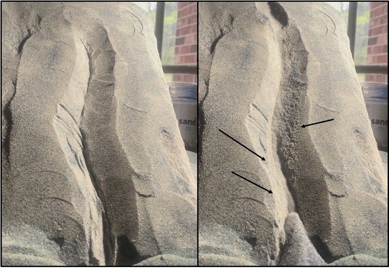
I look at these scoured tracks in lidar imagery all the time, and I wondered if might be possible to use granular analog materials to create similar eroded tracks in a sand model. Using a sand-flour mixture to make a cohesive slope was a V-shaped channel sculpted into it, I triggered slides of glass microbeads at the channel heads. The microbeads tend to fluidize when they are moving and colliding with one another, producing a dry analog for a natural saturated flow with lots of rocky debris. As seen below, the model flow does indeed erode the underlying slope and entrain the eroded material, added to the flow volume. I roughened the bottom of the initial channel to make the results of the scouring more noticeable.
This is a simple model, but the effects of the flow on the initial slope condition are easy to see. Greater flow/track length would be good, but keeping the cohesive slope material stable on top of the tilting model base is difficult, and only gets more difficult as the model is scaled up. The flow is the most erosive towards the lower part of the model channel, where it is most concentrated. The image below provides a nice start-to-finish comparison.
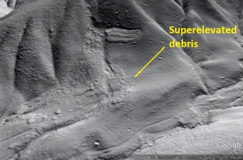
Debris flows also surge up slope due to their momentum as they move around channel bends. Evidence of this process is visible in lidar imagery, as in the case of the 1995 debris flow shown below, which occurred near Graves Mill, Virginia. Like the previous example, vegetation is yet to fully recover. The transparent red outline shows the limit of scouring by the flow; the thin blue line shows the present-day water channel. Arrows show where momentum of the flow caused to it to run up, or superelevate, on the slopes.
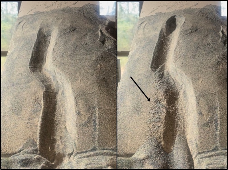
The same model flow setup will produce some amount of the superelevation effect, along with scouring, if a curving initial channel is constructed. The GIF below shows one experiment.
The model flow superelevated twice, with the most obvious scour indicated by the black arrow. Removal of the surface lumps and bumps from the starting channel (left) is apparent in the post-flow appearance (right).
Another Graves Mill lidar example is shown below, with arrows indicating subtle evidence of scour due to superelevation of the flow. More on this event and its lidar signature can be found at this link.
Another curving channel example is seen below. This one also superelevated twice, with the second superelevation leading right into the zone of deposition. These flows don’t go very far once they leave the steep portion of the slope/channel because they are dry…see the video link at the end.
Comparing pre- and post-flow imagery shows erosion by the flow clearly, with initial texture in the channel scoured away where the flow was most concentrated.
A final example of flow behavior from McDowell County, North Carolina, shows how flow material can completely overwhelm a shallow channel due to volume or velocity and spread out over a flat slope. The transparent red area shows surfaces affected by the flow; whether the textured area to the right of the channel is eroded or holds deposited material (or both) is not entirely clear.
The following GIF shows this type of movement, with “spillover” debris leaving surface texture outside of the pre-formed channel.
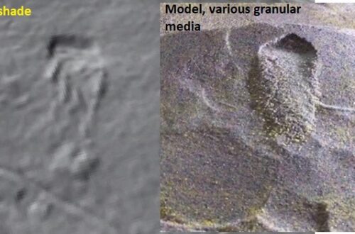
Situations like this are actually quite common in the southern Appalachians, particularly with flows that occurred during the most extreme precipitation events (more than 10 in/25 cm of rain in less than 10 hours). Storms that generate this much rainfall have produced several “splashy” flows in which rock and boulder debris has surged out of channels and cascaded across generally planar slopes, often for significant distance. The lidar signature of this type of movement can be subtle, but it is identifiable once you’ve seen it. My main purpose in making models like these is to support pattern recognition in remote sensing, and this model came out very nicely.
These out-of-channel surges are not dramatic in lidar, but they do promote thought about debris flow mobility and just what parts of steep slopes are actually safe during extreme rain events.
The following video link shows footage of all of the models, along with the deposits left by the models. Because they contain no fluid, the flows grind to a halt fairly quickly when slope and velocity decline. Most deposits end up preserving a “jet” of microbeads within a broader area of less mobile material, including what the flows scour from the channels. In real, saturated flows, the jets of microbeads would be actual fluid material, which would blast through the deposit to leave a channel flanked by levees of coarse debris.
-
Another track left by huge boulders visible with lidar, Big South Fork National River, Kentucky
by Philip S. Prince
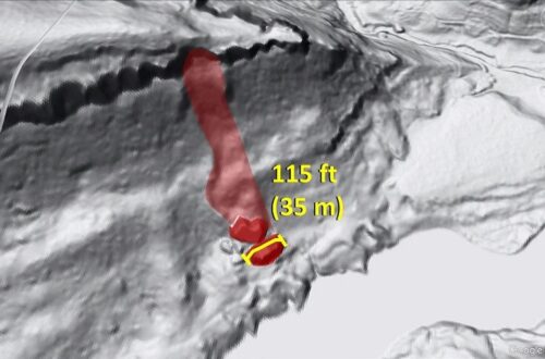
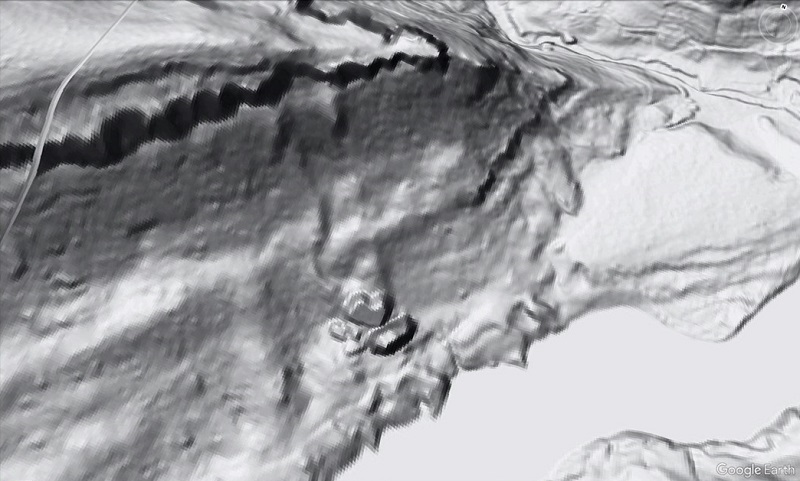
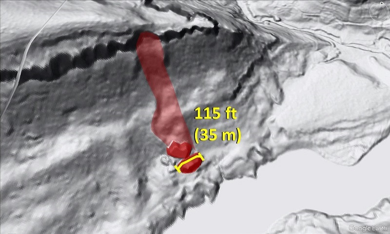
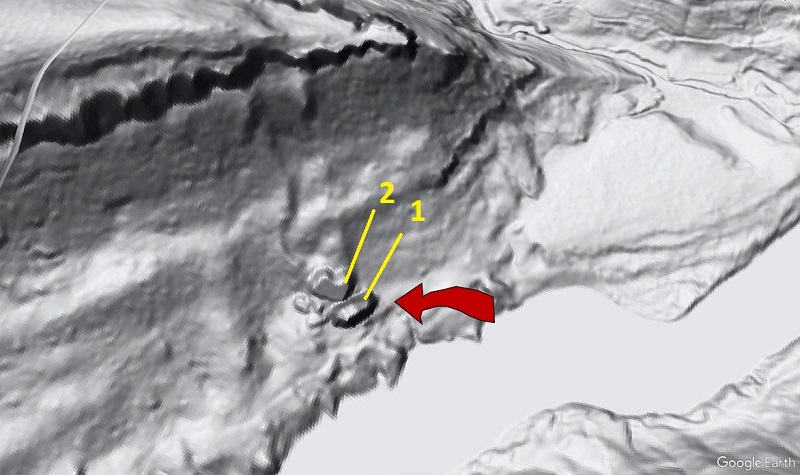
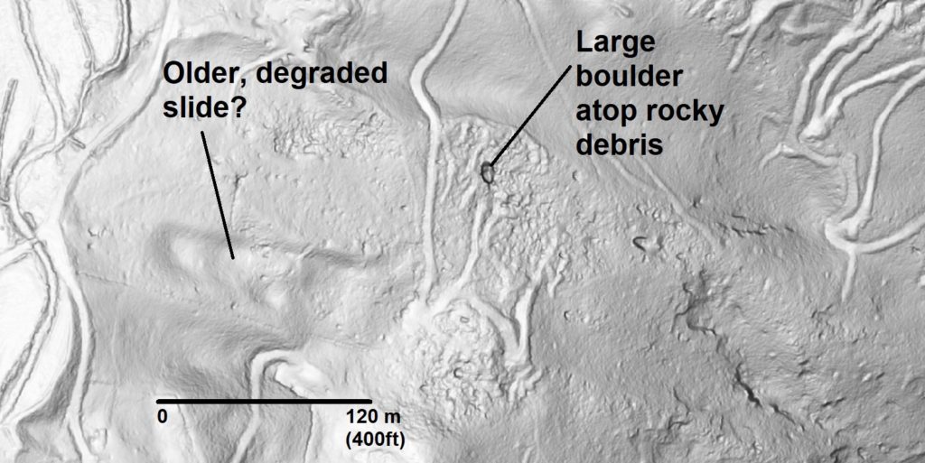
As rugged and/or high topography in Appalachia tends to result from outcrop of particularly hard and weathering-resistant rock, steep slopes in the Appalachians are often home to boulders, some of which are quite large. An interesting aspect of the boulders is that very few have been known to slide or roll into place since folks started recording such things, and they very, very rarely show visible tracks or paths downslope in lidar-derived imagery. The question of how the boulders got to their resting place is legitimate (more on this below), but sometimes, lidar serves up a nice answer, as in the case of the two huge (115 ft or 35 m long) McCreary County, Kentucky, boulders shown below. The boulders and their track are highlighted in the lower image for comparison to the bare lidar.
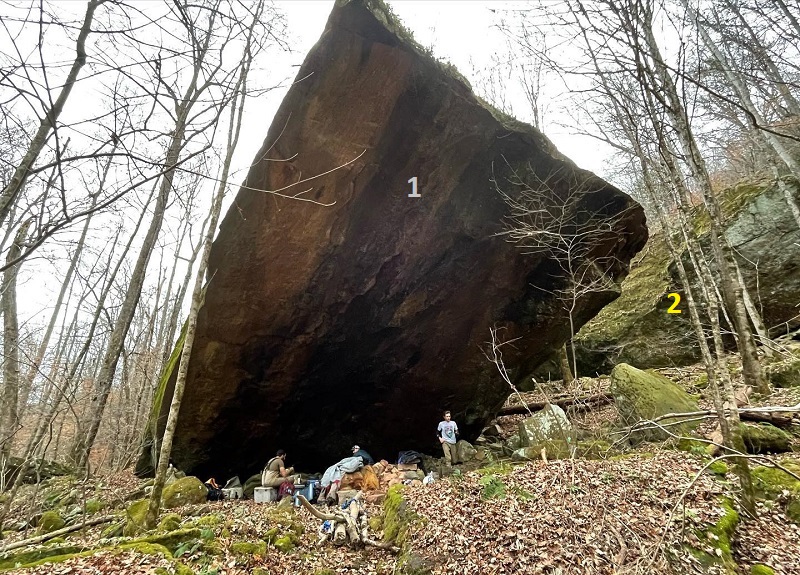
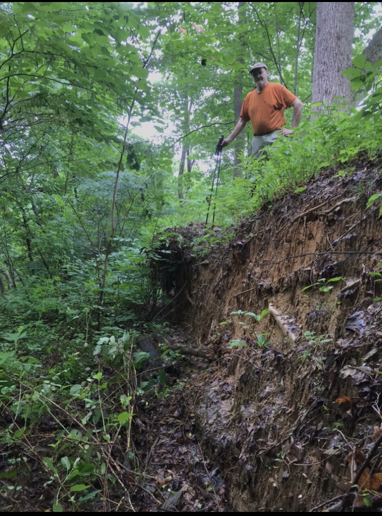
I got tipped off to this feature when a friend posted a shot of the lower boulder (the one with the measurement bar, above) on Facebook, shown below. It’s an impressive image, and gives a sense of the boulder’s scale relative to human observers. The second image below uses a large arrow to show the general perspective of the photo, which also gives a glimpse of the second boulder (2) in the background.
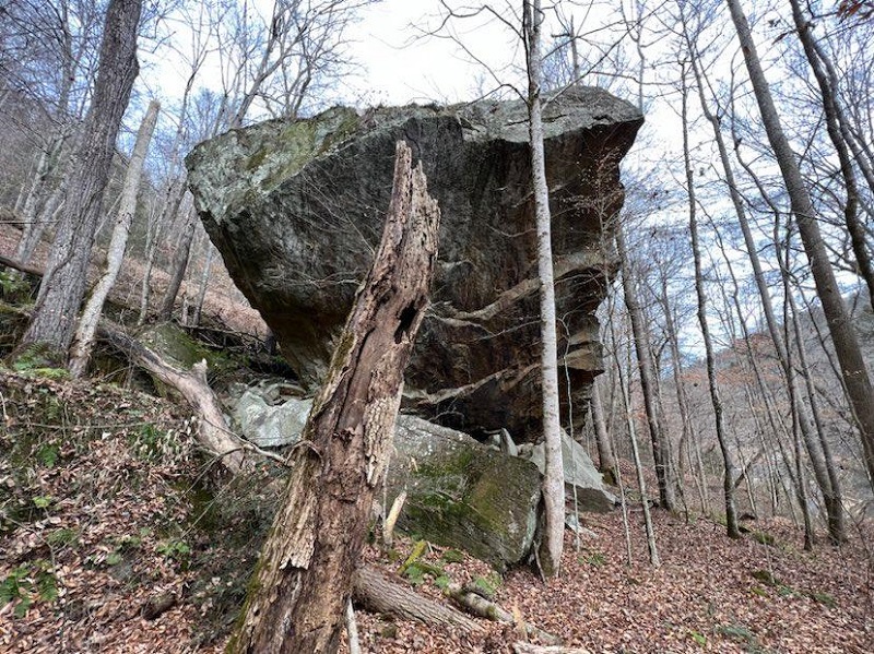
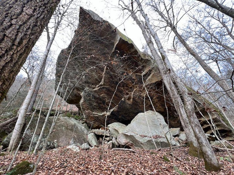
The path carved by the boulders is as wide at the boulders’ long dimension, which suggests (I think) that they slid into place instead of tumbling, without turning much on the way down. The plowed-up path appears to be about 10 ft (3 m) deep, but is entirely re-vegetated with no obvious distinction in vegetation. The additional photos of the boulders below show that they are now just “part of the forest,” so to speak.
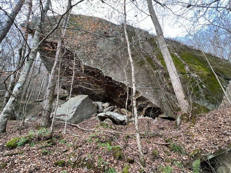
The boulders are Pennsylvanian-aged quartz-rich sandstone (possibly Rockcastle Formation?), so they are physically and chemically very tough and look to be well-preserved. I have not personally been to these boulders, but it’s likely that a geologist could easily establish which sides of the boulders were facing up and out (the old cliff face) prior to detachment and emplacement. Reddish-brown oxidation on the underside of the boulder in the image above might be a clue to this sort of interpretation, but I’m not sure.
The boulders are located along the Big South Fork National River, which carves a steep gorge through the Pennsylvanian-aged geologic section in northern Tennessee and southern Kentucky. The river itself is full of boulders in this area, but most are processed out of the lidar data. The Google Earth image below shows the river in the vicinity of the giant boulders, and is paired with a matching lidar overlay for reference to the tracked boulders.
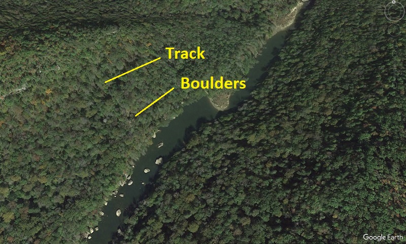
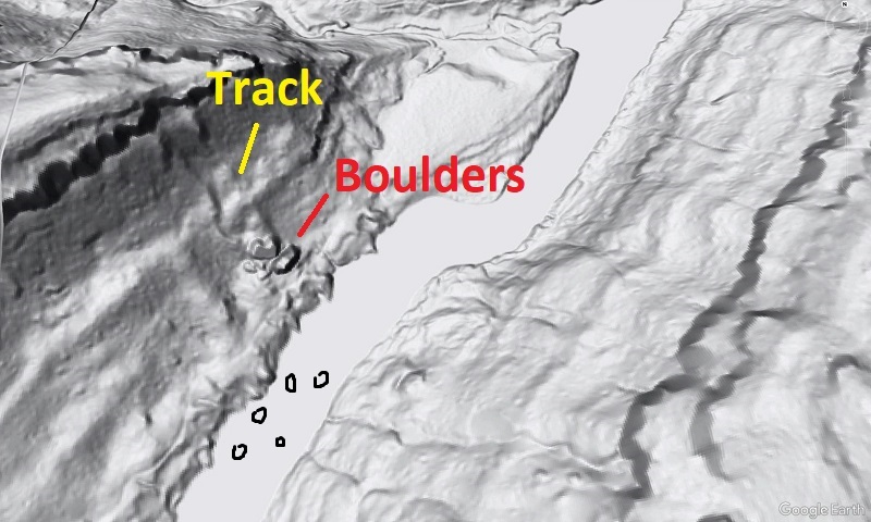
This “tracked boulder” example is particularly interesting because it provides direct evidence that the boulders traveled overland to their resting place, likely in one big event. Falling, sliding, or tumbling during a major failure are not the only ways boulders might move downhill. Rapid weathering of weak or soluble rocks below the cliff line might allow pieces of the cliff line to be gradually lowered as the underlying bedrock weathers away, causing a former cliff line position to decay into a line of scattered boulders. Boulders might also slowly creep downslope if the underlying soil or rock are sufficiently unstable, particularly during wet climatic patterns or aggressive freeze-thaw cycles. I think (but am not entirely sure) that both of these non-falling processes are either documented or suspected in cases of apparent large boulder movement elsewhere in the world. In this Big South Fork case, however, the physical evidence suggests the boulders failed and slid in an impressive event and plowed a 3 m (10 ft)-deep path down the slope. Knowing that boulders can and do move like this in the Cumberland Plateau landscape is useful to understanding potential hazards and how best to interact with the landscape, particularly from an engineering standpoint.
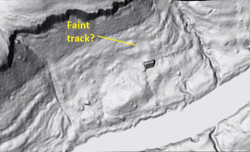
Understanding why more boulder tracks aren’t visible in a region as bouldery as the rugged parts of Appalachia (throughout its provinces–not just sandstone-capped Plateau areas) is another interesting question. Plenty of large boulders are found near the tracked example discussed here, but none show any obvious surficial evidence of their path downhill. One 28 m (~90 ft) long boulder immediately downstream might be argued to show a well-weathered track, but detailed analysis of soil in the possible track relative to surroundings might be necessary to confirm it. I don’t think the lidar-derived imagery alone is convincing enough.
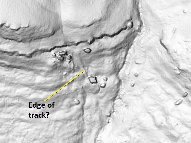
The only other good candidate I have seen in the Cumberland Plateau occurs about 200 km (125 miles) southwest, across the Sequatchie Anticline from Chattanooga, Tennessee. This 20 m (65 ft) boulder, also of Pennsylvanian sandstone, appears to have left a short track, though its point of origin is unclear. A scar shaped like the boulder’s upslope edge may be visible just uphill, suggesting a small amount of travel that occurred after the boulder was separated from the outcrops upslope.
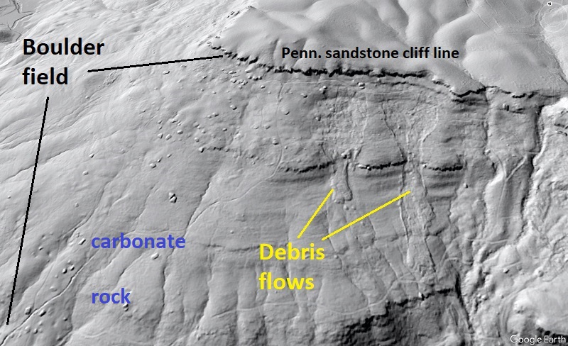
Many Cumberland Plateau slopes are absolutely covered in boulders, but are comparatively gentle (less than 20 degrees) and seem less likely to support rapid and significant boulder travel by slide or rockfall events. The slope shown below is a good example. It is covered with 15 m (50 ft) boulders that suggest association with the cliff line, but just how they ended up so far from the cliff line on a <20 degree slope is another question. Here, dissolution of carbonate rock may indeed play a role, suggesting evolution of the landscape visible in the image represents a very complex interplay of processes. The cool debris flows are an added visual bonus–did they mobilize any boulders?
This post is Cumberland Plateau-focused because the rock types and structure that produce its landscape make visually impressive boulder examples, but the questions raised here apply to the Appalachian Plateau to the north, the Valley and Ridge, and the Blue Ridge and westernmost Piedmont. All of these provinces host many impressively boulder-covered slopes, and seldom do the boulders offer any evidence of when or how they ended up where they are today. Understanding boulder separation from outcrops and downhill movement goes beyond just being interesting–it can improve understanding of how climate history shaped the landscape as well as how dynamic hillslopes can be. As lidar-derived imagery offers a new way to look at boulders on forested slopes, geologists are likely to greatly expand understanding of Appalachian hillslope evolution in coming years.
-
“Blowout” landslides and the lidar signature of extreme Appalachian rainfall events
by Philip S. Prince
On the night of June 27, 1995, the Albemarle County, Virginia, mountainside shown below received an exceptional amount of rainfall. No one knows how much, but a nearby rain gage recorded ~ 11 inches (28 cm) of rainfall with only 2 hours…the rain event continued for several more hours. Unsurprisingly, a tremendous number of landslides resulted. The slides are clearly visible in this lidar hillshade image, and those marked with yellow arrows are of particular interest in the context of the storm’s outrageous precipitation rate and total, which likely reached 30 inches (76 cm).
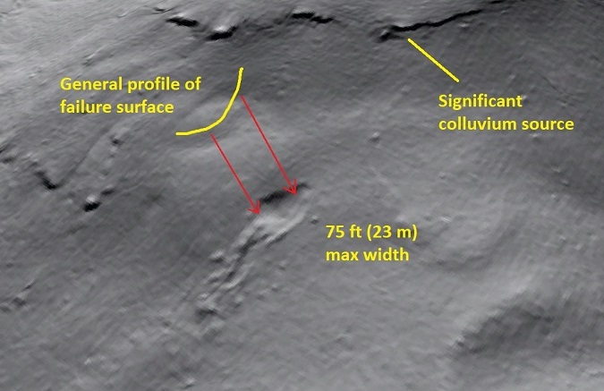
The slides highlighted by the yellow arrows are examples of what William Eisenlohr, Jr., called “blowouts” following a July 1942 storm that produced similar features near Port Allegany and Smethport, Pennyslvania, as a result of similar rainfall rates and totals. Below, a detail of the slide at upper left in the image above shows particular details of the type of failure that inspired the unusual “blowout” name: a curved failure surface and arcuate scar, no erosive track, no intact slide block, and debris spread as a sheet over the slope below. Notably, much debris is missing; the deposit visible below certainly doesn’t account for the volume removed from the scar.
These “blowouts” and their association with extreme Appalachian rainfall events (more than 10 inches (25.4 cm) in under 10 hours) offer up an interesting story about hillslope response to extreme rainfall and the very 21st century ability to see that response with 1 meter (or better) resolution lidar. Linked below is a full-length post I recently wrote about these slides on the Appalachian Landslide Consultants, PLLC, page, which shows blowouts related to atypical storms in several Appalachian settings:
Link to original Appalachian Landslide Consultants post
I usually don’t base a post on this site about external material, but in this case pasting a link is admittedly more appealing than re-posting all the figures and text. The Appalachian Landslide Consultants page also allows images to expanded to full screen with a click, which is a plus. Original reports about the slide events are linked in the full-length writeup, and I personally enjoyed checking out the sites highlighted in Eisenlohr (1952) and Hack and Goodlett (1960) (shown below) with 2017 lidar!
-
Lidar imagery reveals details of debris flow movement in the eastern Blue Ridge Mountains of North Carolina
by Philip S. Prince
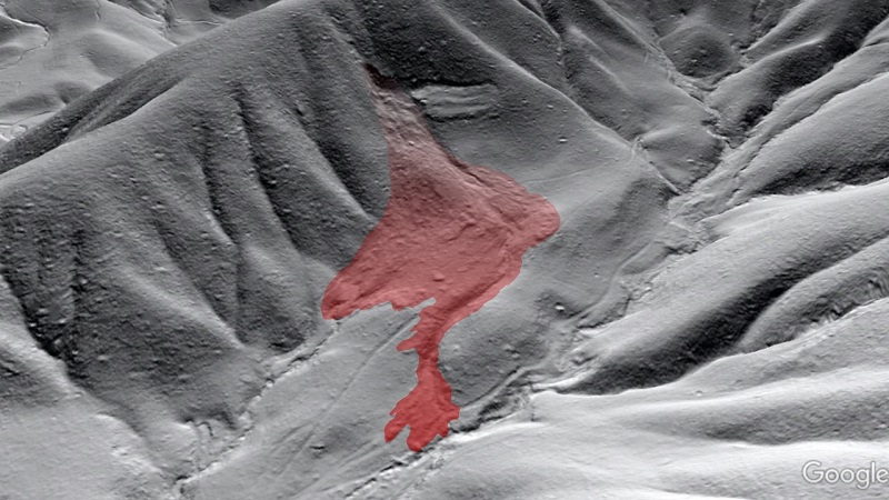
Lidar-derived imagery is a remarkable tool for showing how rock, soil, and woody debris moved over the landscape during old debris flow events. Understanding how this material moves is a key aspect of understanding present-day debris flow hazard. Lidar imagery provides a way to track downslope material movement of old flows that is otherwise difficult or impossible to see in the field, which is particularly significant in forested Appalachia. This post highlights some interesting debris flow styles and paths now hidden by vegetation in Pisgah National Forest in Transylvania County, North Carolina. I have tried to label relevant features without obscuring details of the deposits, which are quite subtle but notably distinct from the rest of the landscape once you see them. The GIF below uses a transparent polygon to highlight a flow path and deposit on the north side of the Davidson River southwest of Brevard, North Carolina. This one is a good starter, as details of the initial failure and subsequent flow path are reasonably easy to pick out.
This flow appears to have resulted from the partial breakup of an intact landslide block, much of which did not flow and remains clearly visible as a detached rectangular feature on the slope. For a sense of scale, the intact rectangular block is about 200 ft (60 m) across. Due to the shape of the landscape, the debris flow resulting from breakup of part of the slide block quickly reached the smooth but sloping valley floor, where it spread out before re-channelizing toward the bottom of the image. The flow had sufficient momentum to superelevate (move at an angle to the slope instead of straight down the slope) and bend away from the faint upper channel before the material turned back towards the channel. A faint dashed yellow line highlights the curve in the levee-like deposit edge as it bends back onto a direct-downslope path.
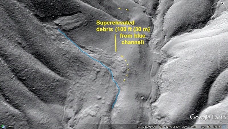
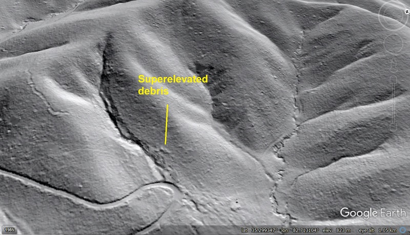
Superelevated debris extends about 100 ft (30m) across the ground surface from the faint upper channel, which is highlighted by the blue line.
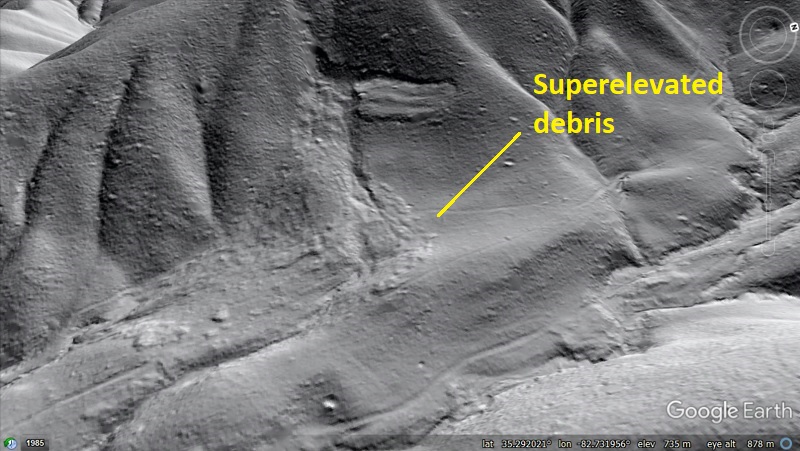
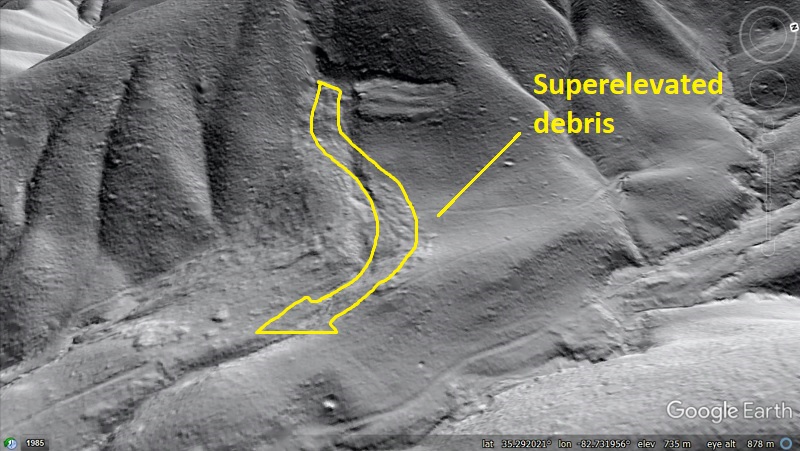
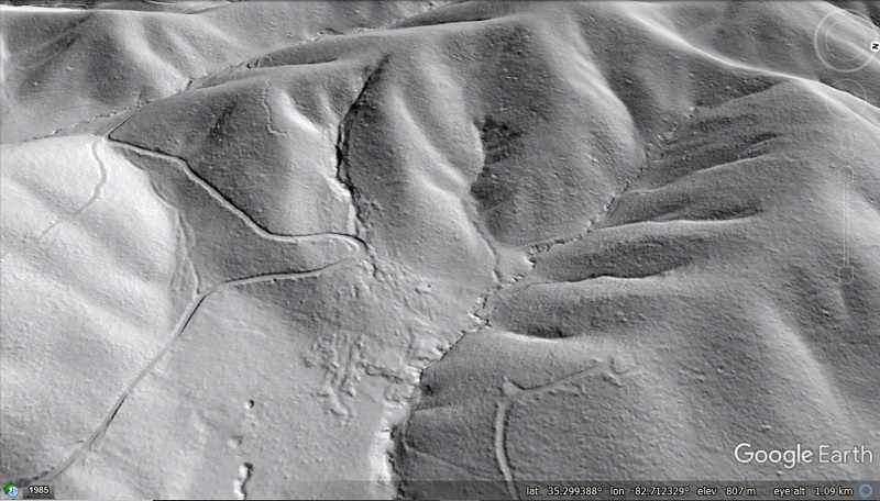
A head-on view (below) gives more context to the superelevated debris, which moved oblique to the slope of the valley before losing momentum and following the slope. The second image offers a basic illustration of how the debris “banked” its way downslope.
Lobes and sheets of deposited material, along with one large boulder, are visible further downslope. This slide-to-flow was obviously quite fluid and mobile despite the modest relief between the failure point and the sloping valley bottom. After traveling overland in the area shown above, portions of the flow re-channelized and continued downslope. The deposit terminates at a ground length distance of 1.180 ft (360 m) from the failure point, having descended about 265 ft (80 m). The transparent polygon in the image below covers the full extent of the deposited material visible in lidar.
2.2 miles (1.3 km) to the east, another subtle debris flow deposit is visible spreading across a gently sloping valley floor. The GIF below shows the extent of the deposit, which resulted from a flow originating in a small channel upslope. No clear initiation zone is visible above the head of the channel, suggesting the flow began within colluvium stored in the small channel itself. The deposit highlighted by the transparent polygon is about 280 ft (85 m) wide at its widest.
This flow also occurred in reasonably modest topography, descending about 230 ft (70 m) over a ground length of 1,000 ft (~300 m) from the apparent initiation zone to the toe of the deposit. Near the upper end of the polygon, a line of superelevated debris is visible on the otherwise smooth hillslope. This material was likely deflected onto the slope by the slight bend in the to the left of the superelevated debris as shown in the image below.
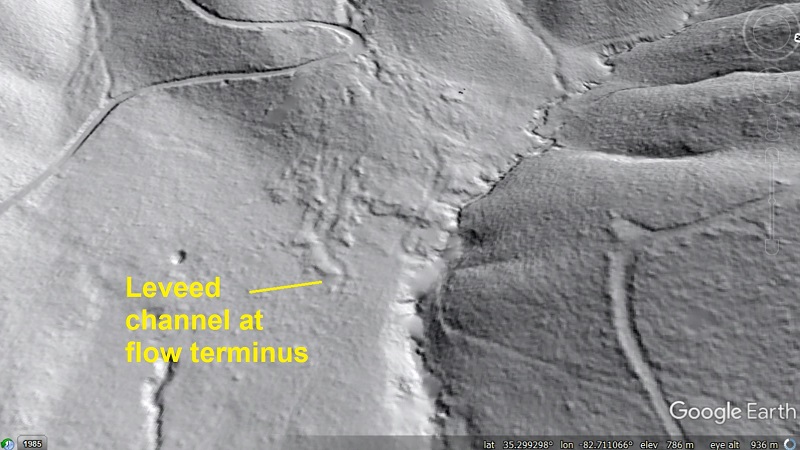
While the deposit from this flow is more subtle than the previous slide-to-flow feature, it is definitely visible once you know it’s there. The lowermost portions of the deposit stand out nicely against the comparatively smooth valley floor. Much of this deposit is draped across a faintly convex area, which is visible just below the logging road switchback that cuts into (and obviously postdates) the deposit.
The leveed channel at the tip of the deposit is particularly interesting, with the outlet for fines and flowing water clearly visible.
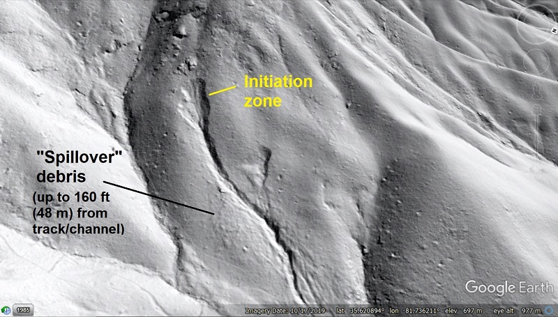
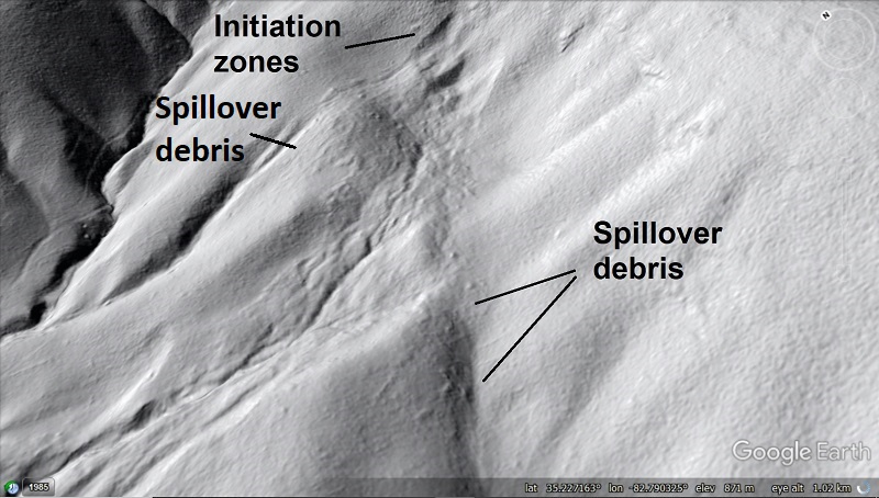
About 6 miles (~10 km) southwest, a comparatively complex debris flow deposit can be seen on a slightly larger and more rugged hillslope. This deposit spilled out of the narrow, shallow “trough” that steered it in two places, though the bulk of the flow reached the stream below after traveling a ground length of ~1,200 ft (~364 m). The flow descended ~380 ft (115 m).
The “spillover” zones result from the unusual topographic shape of the hillslope, where three faint channel heads are located in close proximity to one another. This failure was also quite voluminous; the failure scars are about 25 feet (just over 7 m) deep and 260 ft (80 m) wide. An oblique image (below) puts both “spillovers” into topographic context. The second image uses yellow arrows to give a sense of material movement in this failure. I have actually visited this feature in the field, and the spillover material would not be noticeable without lidar-derived imagery of this (0.5-meter) resolution.
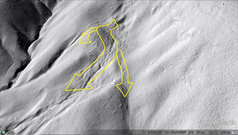
These debris flows are particularly interesting to study because they are distinct from many other debris flows in the region, whose downslope travel is strongly controlled by topographic channels along much of their length. The flows shown here experienced less topographic control and presumably less “bulking up” by collecting soil, rock, and wood along their paths. Despite their lack of extended channelize flow paths, the spread of these flows, along with their mobility in close proximity to their initiation zones, provides an interesting glimpse into the physical dimensions of possible impact zones related to this type of slope failure. The age of these failures is unknown, but they likely occurred in 1916 during an extreme tropical precipitation event in the area. They are completely obscured by forest cover today, and the information about slope failure effects that they preserve would be completely lost without this lidar data set!
You May Also Like
Pleistocene Coastal Plain sand dunes and the value of pattern recognition in LiDAR interpretation
LiDAR reveals the cloth-like appearance of a “wrinkled” translational landslide
Lidar highlights impressive landslide density on the southern Appalachian Blue Ridge Escarpment, western North Carolina
-
Lidar reveals geologic details of the “worst” coal mine in the Valley of Virginia
by Philip S. Prince
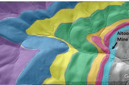
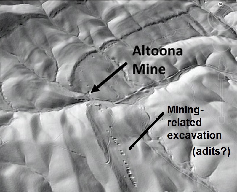
At first glance, the Altoona Coal Mine of Pulaski County, Virginia, seems to be in just the right place. Coal beds in its Little Walker Mountain setting occur just up-section and downhill of a prominent sandstone bed, which forms an obvious “rib” on the slopes of the mountain. The mine was opened right at the base of this rib. This must have appeared to be a great location, as it took advantage of a stream valley to ease construction of a tram railway to the mine. Prospect pits and mine adits leading up to the Altoona’s location are visible in the GIF below. The rib is marked with a pink overlay, with mine workings visible as tiny dots to its right; the image that follows the GIF is a detail of mine workings adjacent to the rib.
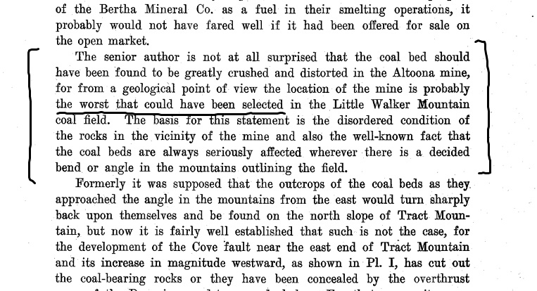
Despite its apparently good location, all was not well at the Altoona Mine. Coal seams in the mine were too distorted and mixed with surrounding rock to be easily extracted, leading to its ultimate failure. Early 20th century geologist Marius Campbell addresses this issue at length in the 1925 report The Valley Coal Fields of Virginia, twice calling Altoona’s location “the worst” in the general area and the obvious reason for the mine’s closure.
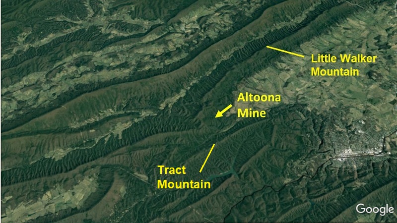
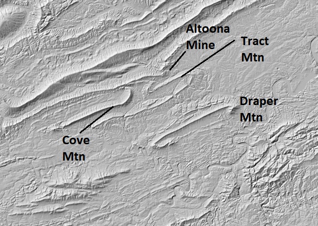
Campbell connected the geologic issues in the mine with its position near a complex ridge pattern that implied large-scale folding in the underlying strata. His focus was on the apparent convergence of Little Walker Mountain and Tract Mountain southwest of the mine’s location. This pattern is visible in Google Earth satellite imagery, and is also quite noticeable from ground level near the mine. Little Walker Mountain, which is typically an arrow-straight ridge, is noticeably buckled in the vicinity of the mine, and Campbell may have seen this feature as evidence of rock deformation associated with the Little Walker-Tract Mountain structural setting.
Campbell was definitely onto something, and he was certainly correct that weak rocks, like coal, focus deformation when surrounded by stronger material like sandstone or limestone. He attributed rock distortion at the mine to “cross-folding,” which appears to be his term for the structures that create the locally buckled appearance of Little Walker Mountain. As it turns out, Campbell wasn’t exactly correct, but accurate interpretation of the area is essentially impossible from field data alone due to limited outcrop. Additionally, no high-altitude imagery was available at the time, preventing Campbell from having a Google Earth-style, satellite-level view of the mine’s setting. Today, lidar-derived imagery quickly reveals the true structural issue at the mine, along with the large-scale context of the distorted coal beds.
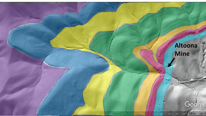
A close look at a 1-meter lidar hillshade image reveals that the Altoona Mine is indeed positioned exactly in a fold hinge. This fold structure is more significant and affects a greater thickness of rocks than Campbell’s “cross fold” concept suggested (more on this below), but it is still subtly expressed, even in the high-resolution lidar imagery. The GIF below overlays color bands onto distinct rock units to highlight the fold, which is very tight and probably faulted. I think the fold is most visible just below and left of center, where the purple and blue bands meet in a V-shaped point. From here, the faint layer patterns can be followed towards the mine. Layers young towards the right; purple covers Devonian-aged rocks, while the mine is developed into Lower Mississippian-aged rocks.
The significant folding near and left of image center appears to die out in the vicinity of the mine, where the sandstone rib that highlights the coal location does not immediately appear offset. An even closer look suggests that the rib is deflected to the observer’s left, indicating that the rib layer and coal-bearing interval are either folded into a very tight syncline or repeated by a minor thrust fault. The mine is located nearly atop this highly distorted area, which nicely explains the messy condition of its coal beds.
Based on these lidar-derived images and my own experience in the area, the structure immediately adjacent to the mine would not be decipherable through field work. Sedimentary rock layers visible in the lidar imagery do not actually produce much surface outcrop; they only create faint bulges on the land surface that require a 1-meter resolution (or better) digital elevation model to see. The fine structural details at the mine are still not completely clear in the imagery, but I would offer the two conceptual models below as explanations of the folding and faulting that produces the observed surface pattern. They are very similar (differing only in terms of a small fault vs. a fold in the mine area), and both would produce considerable distortion of the coal-bearing horizons. The models use a wedge-type geometry instead of a single fault cutting all the way through the affected section. This is a way of reducing apparent offset of the pink sandstone marker bed, which is not obviously deflected to a ground observer or coarse-resolution map user.
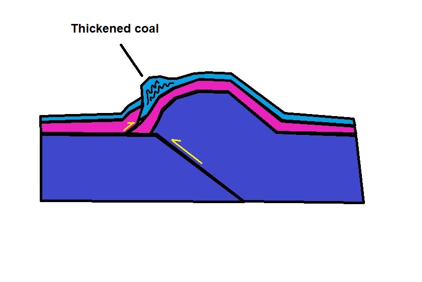
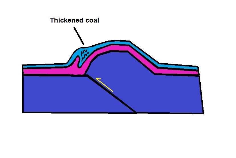
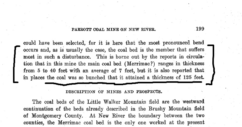
Both models focus shortening into the coal zone and would result in thickened, duplexed coal seams. Thickening of coal beds is one of the details reported by Campbell, with the main coal bed in the mine reaching 125 feet (~38 meters) thick in some areas despite an average thickness of 7 feet (just over 2 meters).
In addition to locally thickening the coal, the tightness of small scale folding in the mine, along with possible faulting, would have broken surrounding sandstone layers and forced pods of sandstone into the more ductile coal. Coal beds in the mine would thus have been observed to be locally atypically thick or atypically thin, and full of fragments of surrounding non-coal rock. As a result, the mine would have been nearly impossible to develop efficiently.
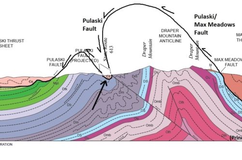
As mentioned earlier, folding around the Altoona mine is not the result of the mine being between Little Walker and Tract Mountains. In actuality, the fold on which the mine is situated has developed along one of at least two thrust fault structures that climb out of the Devonian-aged rocks into the coal-bearing Mississippian aged rocks at the mine. These faults produce the bends or buckles in the Little Walker Mountain ridge and may have accommodated displacement as bedding plane faults in the Mississippian strata, either in the coals themselves or in the overlying Macrady shale. I highly doubt these larger faults would be easily field-mapped either, due to the difficulty of finding meaningful bedrock outcrop where the faults climb upward into the Mississippian layers. Where the faults are operating as detachments or flats within a single stratigraphic interval, they are not readily identifiable even when outcrop is present. The GIF below traces these faults relative to the mine’s location.
While coal extraction was not particuarly successful at the Altoona Mine (and never will be!), the mine’s coal issues highlight a structural scenario that is valuable to structural interpretations of the surrounding areas. Cove and Tract Mountains, the respective left and right elliptical ridges south of the mine, are part of a large structural mass that is difficult to relate to neighboring thrust sheets. Cove and Tract Mountain (as well as Draper Mountain to the south) reached their structural position on what should have been a high-displacement thrust fault, but evidence suggesting this high displacement is hard to find.
Activity on the detachment fault that terminates around the Altoona Mine could help explain some of the “missing” fault displacement, particularly where the additional fault to its north is considered. These otherwise subtle features would largely escape consideration were they not connected to a conspicuously bad coal mine, making the Altoona a geological success long after its closure!
You May Also Like
A mid-1800s description of landslide topography meets 21st century lidar at Split Mountain, Haywood County, North Carolina
Lidar hillshade imagery hints at the location of a future coal spoil landslide

Low-displacement landslides explain unusual West Virginia landscape features visible in lidar imagery
-
A mid-1800s description of landslide topography meets 21st century lidar at Split Mountain, Haywood County, North Carolina
by Philip S. Prince
Earlier this week, I came across a recent article from Kathy N. Ross of The Mountaineer newspaper (Waynesville, NC) describing the “mystery” of Split Mountain, a spur ridge rising above the Fines Creek Community in Haywood County, North Carolina. The article is linked here, and is worth a read in conjunction with this post!
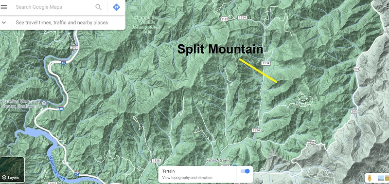
Split Mountain is located north of Waynesville and northeast of Waterville Lake at 35.713630N 82.922300W. The “mystery” specifically refers to episodes of falling rock, formation of lumpy “hillocks” on previously smooth slopes, split and tilted trees, and cracked ground that gave the mountain its name in the mid-19th century. Statesman/geologist/famous North Carolinian Thomas L. Clingman visited Split Mountain three times between 1848 and 1867, describing impressive sights that significantly altered the appearance of the mountainside and conjured up suggestions of an “upheaval” event. Interestingly, none of the features Clingman described are readily apparent today, allowing the mystery to persist.
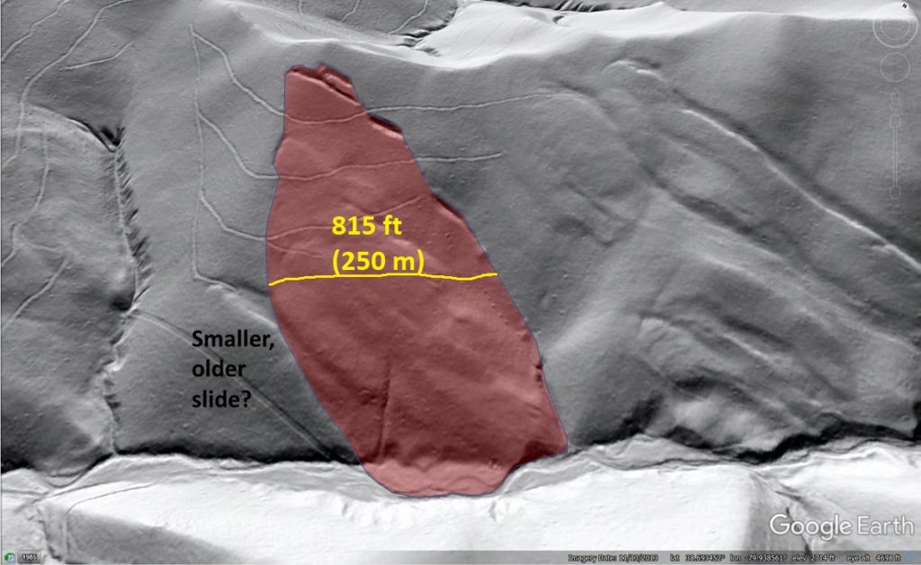
As a geologist working with landslides in western North Carolina, I found Clingman’s accounts to be clear but unintentional descriptions of a large translational landslide on a forested slope. Given the apparent size of the feature and the extremely high resolution lidar imagery I have access to, I thought it might be possible to see the feature(s) Clingman described and give them a bit more context.
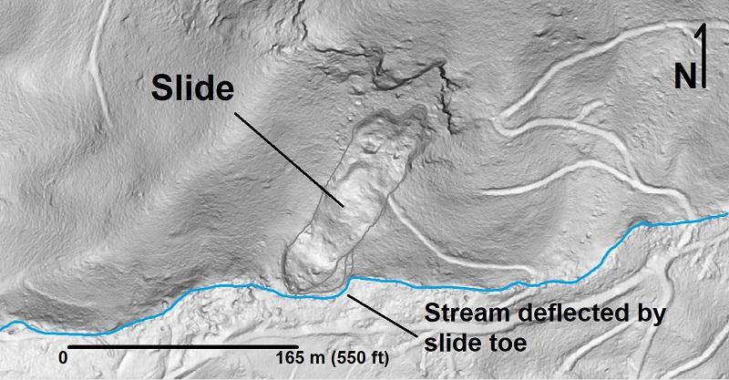
Sure enough, the south side of Split Mountain is home to a significant landslide that could indeed host many of the details that caught Clingman’s eye during his visits. The GIF below shows a slope-shade image of the feature along with aerial photography of the site. The slide is entirely re-forested, and no details of the slide-related landforms would be visible from the valley below. In fact, without the lidar dataset, this slide would go likely completely unnoticed today unless a specifically trained geologist looking for landslide topography happened to hike directly across it in just the right place!
The Split Mountain slide is not particularly large, but it is readily visible in lidar slope-shade imagery. View is to the north in this GIF. The head of the slide is about 90 m (300 ft) above the valley floor, and the cliffs above the slide are about 120 m (400 ft) above the valley floor. Clingman seems to have estimated these distances with good accuracy. Clingman’s observations are readily understandable in the context of landslides, and I have tried to connect them with details of the slide that are visible in lidar imagery and comparable features on a modern slide in the region. In addition to Kathy Ross’ article, a 2008 blog post (author unknown) offers a few more of Clingman’s words that contribute nicely to visualization of the Split Mountain slide. While I cannot, of course, be absolutely sure that what I am looking at is what Clingman visited, I think the chances are pretty good. The only notable disagreement between Clingman’s description and the lidar-visible slide is its size (see below), but I suppose one might expect a bit of exaggeration or at least inaccurate estimation on a forested slope.
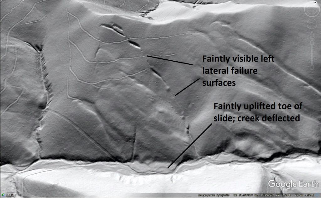
First and foremost, the slide is located on the south side of the ridge, where Clingman said the most striking “evidence of violence” could be seen. The slide is oriented close enough to the north-south trend Clingman described, and, most significantly, it has deflected the stream at the base of the hillside.
Another rockfall feature is present east of the slide, above “ect” in “deflected.” Its age or association with the 1848-1867 events is unknown, but it appears much more weathered and degraded. The slide is quite elongated and mostly translational in its movement, which would have produced long, crisp lateral scarps early in its development.
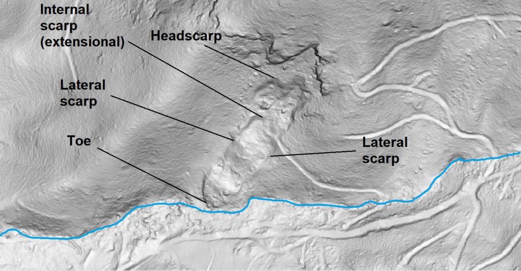
All scarps remain clearly defined in lidar-derived imagery. A lateral scarp in its early stages of development could be the “crack not an inch wide” that “could be traced for a hundred yards.” The photograph below shows an example of this type of lateral scarp-associated crack in Rutherford County, North Carolina, with Appalachian Landslide Consultants geologist Ken Gillon standing across it.
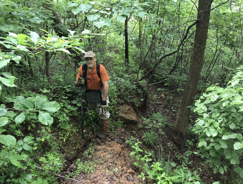
The crack Ken Gillon is standing over extended hundreds of feet on this slide. Note vertical movement associated with it behind Ken…this movement was locally present along the crack/lateral. Material on the left side of the image is moving downslope, away from the image viewer. The elongated crack Clingman described split a large poplar tree, leaving one half remaining standing. Trees can certainly be split by landslide movement, as indicated by the image below. Note that this image is on an extensional headscarp. Presumably, a similar effect could develop along a lateral scarp, particularly in the presence of extremely large trees, which are often absent from modern Haywood County’s slopes after more than a century of timber harvesting.
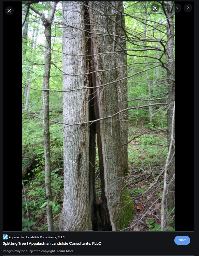
A poplar, no less. Presumably, the example Clingman describes was much larger. Despite largely translational motion, the slide appears to be thick enough to have experienced back-rotation of blocks near its head. Rotated blocks would nicely fit the description of the “hillocks” with tilted saplings that were well established prior to the tilting.
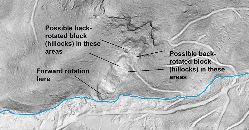
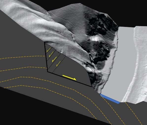
Back-rotated areas below extensional scarps have produced local flats on the slide mass. Since the entire mountainside was sloped in this area, development of the flats would have back-rotated trees that grew straight on the original, steeper ground slope. Block rotation would also create depressions on the hillside, which Clingman referenced on one of his later visits to the site. The conceptual cross section drawing below illustrates a generally translational slide whose main failure surface is roughly slope parallel, but is much steeper at its uppermost breakaway point due to the thickness of the slide. As portions of the slide mass that started above the steep failure surface move onto its less steep portions, they back-rotate and tilt the original ground surface to a flatter slope, often sufficiently to create surface depressions.
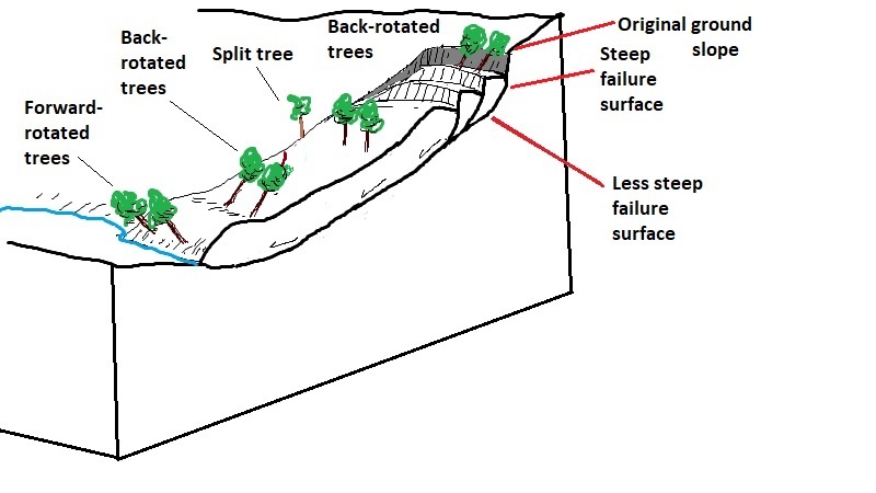
Block rotation occurs in translational slides with adequate thickness when material detached atop a very steep breakaway portion of the failure surface moves onto a more gently sloping portion of the failure surface. The unlabeled trees in the middle of the slide show no tilting because of their location atop a consistently-sloped failure surface. The image below, from the same Rutherford County slide that hosts the lateral crack, shows a large depression with adjacent rotated blocks, whose movement has caused tilting of a large tree at left. These landforms are typical of hummocky topography observed in the upper extensional zones of large slides. Perhaps Clingman saw a scene like this at Split Mountain?
Classic hummocky topography related to block rotation…this is a nice explanation for Clingman’s “hillocks” with tilted trees. Compressional toe features on blocks within a slide, or at its downslope toe, can also systematically tilt trees as shown in the image below. This photo was taken at the downslope, compressional end (toe) of the Rutherford County slide.
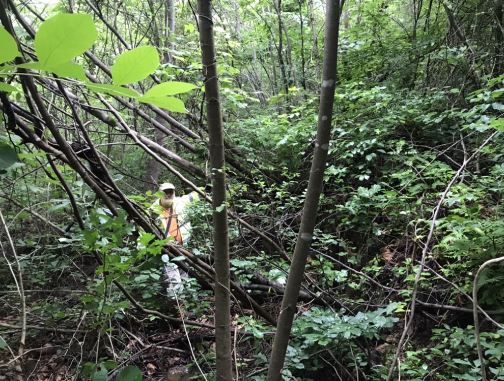
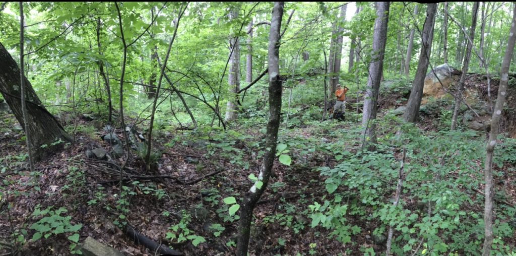
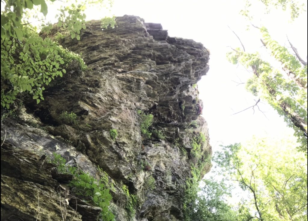
A large boulder seems to be present near the head of the Split Mountain slide, consistent with one of the features which most impressed Clingman. The source of the boulder is unclear, but its location near the head of the slide puts it in a good location to have interacted with “chasms two or three feet in width,” which were probably tension cracks in the upper, extensional portion of the slide.
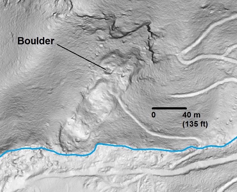
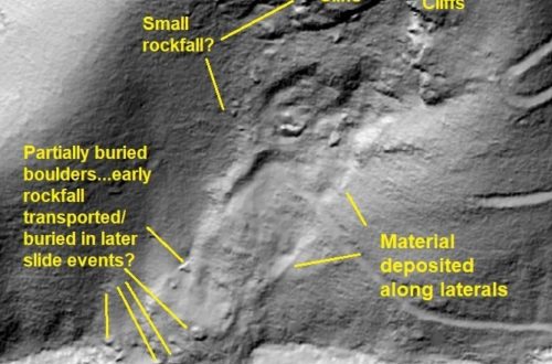
A visit to this boulder might confirm the identity of the slide beyond all doubt should it be broken into three pieces, per Clingman’s description. Where the boulder came from and how far it slid is not clear in the lidar-derived imagery. Clingman described the slide area as having prolonged activity, with rockfall occurring episodically for years before the larger events. Cliffs above the slide are strongly fracture- or joint-influenced, and are certainly a good potential boulder source. I think the shape of the outcrops of the slope suggests a dip slope geometry, which would further favor rockfall (and could explain the slide itself). Early rockfall deposits may have been subsequently transported by later sliding or buried by later addition of material; Clingman references the continually changing appearance of the slide, indicating ongoing activity. The hillshade image below shows some of the boulder locations with a bit more detail than the slope-shade imagery.
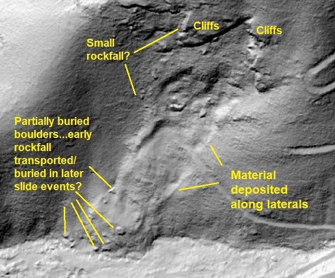
Hillshade imagery sometimes shows added detail of very subtle landscape features, like the trails of material deposited along the laterals of the slide zone. Given boulder distribution and burial, it seems likely that this feature did indeed experience many episodes of failure. The north side of Split Mountain also hosts extensive boulder deposits that are easily visible in lidar-derived imagery. Estimating the relative age of the deposits with respect to the slide on the south side of the mountain is impossible, but the extent of the deposits and the appearance of their source outcrops at the ridge crest, rockfall has been active for some time. Very large boulders are occasionally involved, as evidenced by the example below.
The large boulder shown here sits atop a thick deposit of rocky debris sourced from outcrops upslope (lower right in the image). Perhaps the most interesting question relating to Split Mountain is whether the “shocks” referenced by Clingman and local residents describe the slide events themselves, which appear to have been surprisingly rapid for a somewhat intact slide, or small earthquakes that led to the slide events. The excerpted text I have read is not clear, but it at least suggests that earthquakes large enough to be felt by residents in the area might have preceded or actually caused the slides. Kathy Ross’ article references other accounts of tremors and “cracked mountains” southwest of Split Mountain, but these, too, may have been mistranslated over the years. Split Mountain also invites comparison to the 1874 events at Rumbling Bald in Rutherford County, where seismic events followed by or associated with slope movements appear to have occurred.
From my own perspective, I am interested by the lidar appearance of the Split Mountain slide with respect to its age, assuming it is the right one. Estimating landslide age in the field and remotely via lidar is tough, and is ultimately a somewhat subjective judgment call. A field visit to this slide would be very useful, particularly in terms of seeing how scarps and cracks degrade over a known time interval (check out the last image).
Clingman’s observations also highlight the importance of qualitative understanding of mass movement and its consequences. He probably never watched any sort of landslide happen (or slowly develop), which is certainly a hit-or-miss game in Appalachia today. Even if he had interacted with some sort of large slide event, it would have been almost impossible to have a vantage point to watch the movement and its effects on the slide mass. He also had no way to view the slide from above or without considerable obstruction by trees and vegetation (enter: lidar). As a result, he attributed the surface features he saw to a force pushing up from below, possibly in the way soil expands and cracks when lifted upward by a shovel. He ultimately settled on the expansion of subterranean gases as the cause of the Split Mountain events. Indeed, vertical offset along extensional scarps could give the impression of “upheaval” instead of rotation or relative subsidence, as evidenced by the photo below from the Rutherford County reference landslide.
If you weren’t versed in landslide topography, it might not be obvious whether land moved up or down if you saw something like this… Today, the perspective provided by lidar-derived imagery, an endless supply of YouTube videos, and other approaches such as physical modeling allow geologists to become familiar with the sometimes surprising types of landforms that develop due to slope movement. The small physical models shown below illustrate ground slope tilting and the complex fracture patterns that can develop in the extensional portions of largely intact landslide masses.
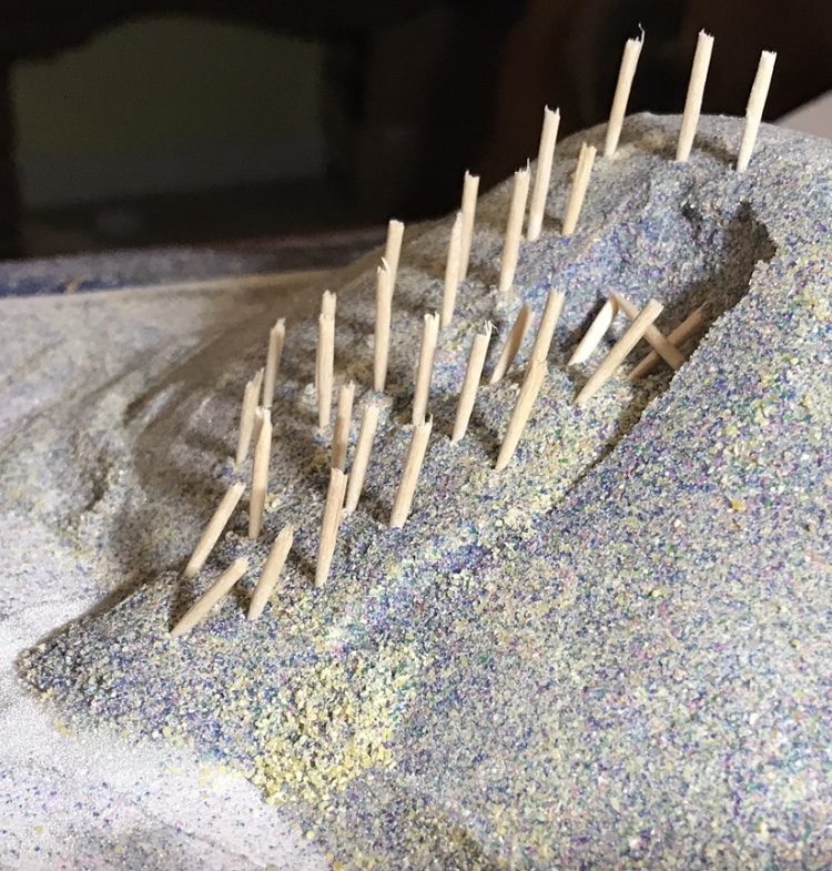
Toothpicks represent trees on this model translational slide. Toothpicks back-rotate at the head of the slide, where the breakaway portion of the slide mass moves onto a less steep glide plane (see the conceptual drawing a few images back). Back-rotation also occurs where the toe of the slide moves out onto the flat surface at the base of the model slope. Within the slide mass, little rotation occurs, and the toothpicks remain as they started. 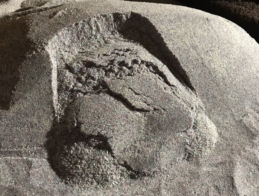
This model slide shows complex patterns of cracking in the upslope portion of the slide mass. In the Appalachians, this basic understanding of landslide-derived landforms is particularly important, as heavy vegetative cover makes interpretation of landslide-associated topography even more difficult. Clingman’s account clearly shows he faced the vegetation challenge on his visit to Split Mountain, but he was able to use tree deformation to his advantage in describing the details of ground movement he observed. While he may have missed the mark on his interpretation of the features, his attention to detail in recording the relevant features of the landscape was right on target, and his account was immediately understandable to a geologist in 2021, over 150 years after he wrote it!
You May Also Like
Low-displacement landslides explain unusual West Virginia landscape features visible in lidar imagery
Lidar highlights impressive landslide density on the southern Appalachian Blue Ridge Escarpment, western North Carolina
Lidar imagery reveals details of debris flow movement in the eastern Blue Ridge Mountains of North Carolina
-
Lidar unboxing day: A few southwest Virginia treats within ~1 hour of Blacksburg and Virginia Tech
by Philip S. Prince
I always look forward to my first look at high-resolution lidar imagery from a familiar area. Last week, I took time to check out some some new-to-me imagery from areas surrounding Blacksburg, Virginia, where I spent about 10 years studying and then teaching at Virginia Tech. I found the following features particularly interesting, as I have regularly viewed or even walked across all of them without appreciating their presence!
- Huge, historically (<100 years) or currently active debris slide, New River above McCoy Falls, Pulaski County
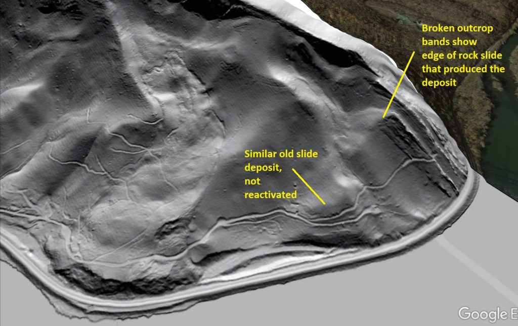
This slide, which resembles a glacier creeping down towards the river, has developed in the debris pile produced by a large rockslide on Walker Mountain. The rockslide laid bare white cliffs of Tuscarora Sandstone that I have always heard called “White Face.” The rockslide is ancient (Pleistocene?), but activity in the resulting debris pile is much younger. The GIF below shows the slide and its topographic context. White Face is visible at the very top center in the aerial photo image. The curving path of the slide can be appreciated from this perspective. I have looked across the river at this area hundreds of times, so this 1-meter hillshade view is very satisfying!
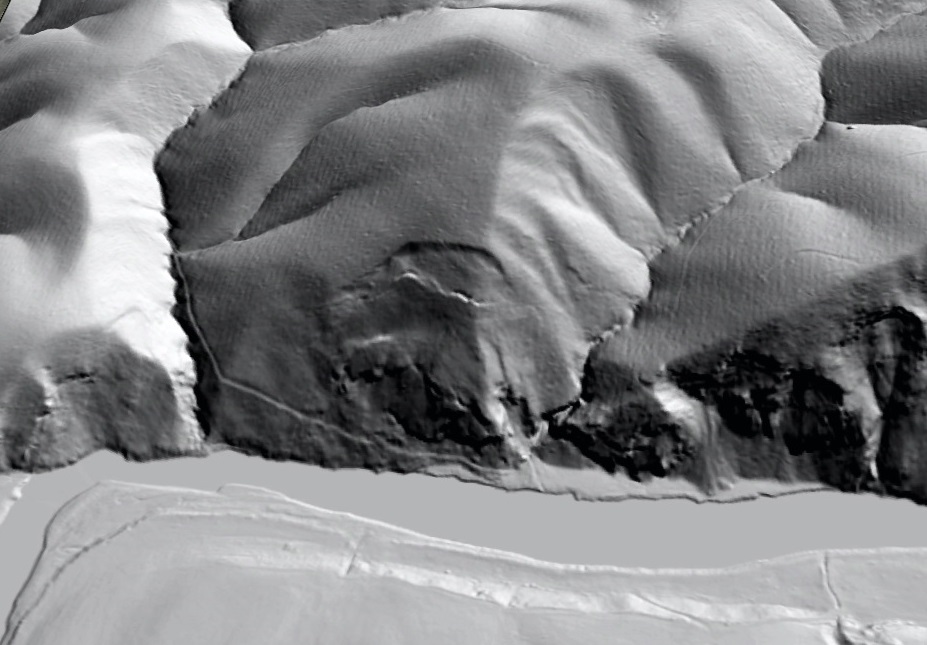
To me, the most striking feature of the slide is the crispness of its lateral scarps and headscarp. They don’t appear to be very large, but remain very crisp and well defined, suggesting recent or ongoing activity.
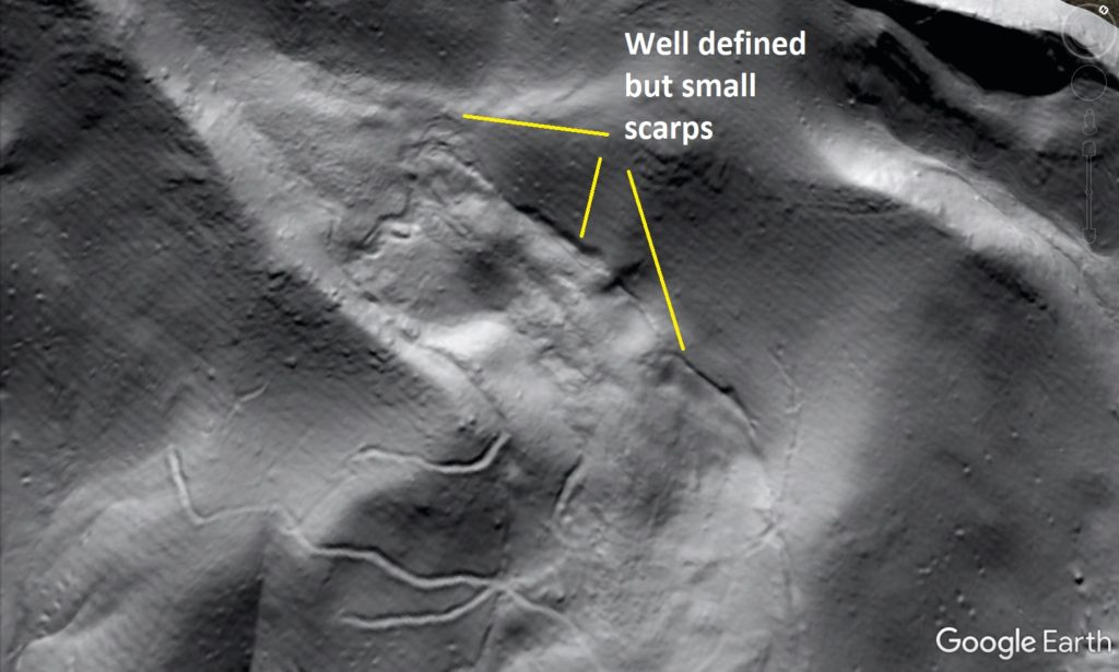
The edge of the slide can be seen cracking along the left-lateral scarp as material pushes up and out of the topographic low that holds the debris deposit.
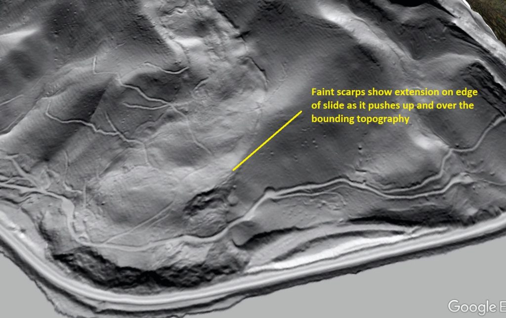
I can’t personally speak to the movement history of the slide, but I suspect that removal of a portion of its toe to construct the railroad running along the river may have led to reactivation. A smaller slide to the north (right side of the image) was not altered by railroad construction, and looks very old and stable compared to its large neighbor.
2. Rock blockslide along Big Reed Island Creek, Pulaski County
This slide has experienced little displacement, but lidar reveals an impressive graben that is forming as a large mass of Hampton Shale (really a slate or phyllite here) bulges outward from the riverbank as it is undercut by Big Reed Island Creek. The slide and graben are at the center of the image below.
The graben and slide are, unsurprisingly, invisible without a lidar-based image.
The graben is quite large compared to the overall scale of the slide. I think this indicates that the basal sliding surface slopes less steeply than the land surface, meaning the slide mass is thick and deep, particularly at its upslope end. The block diagram below attempts to illustrate this idea.
This slide is included on the Hiwassee quadrangle geologic map (linked here), and structural data indicate the failure is occurring along the crest of an anticline that plunges northeast. The basal sliding surface could therefore be a bedding plane/foliation plane failure whose low dip is an expression of where it sits within the fold structure,. The orange form lines in the diagram generally indicate layering orientation as it might appear on this cross section cut, which is at an angle to the fold axis.
I actually went to the foot of this slide with Virginia DGMR geologist Matt Heller during a canoe transect of the map area in June 2019. The poor photo below shows what the downslope end of the slide looks like, right above Big Reed Island Creek. This huge outcrop sheds plenty of rock, and does not feel like a place you would want to stand around for too long.
3. Buck Hollow Ridge rock slope deformation, Macks Mountain, Pulaski County
This slope movement is not far from the Big Reed Island Creek feature, and occurs in Erwin Formation quartzite just up-section from the Hampton Shale. Sub-surface failure within the Hampton Shale may have actually caused the movement, but I don’t know for sure.
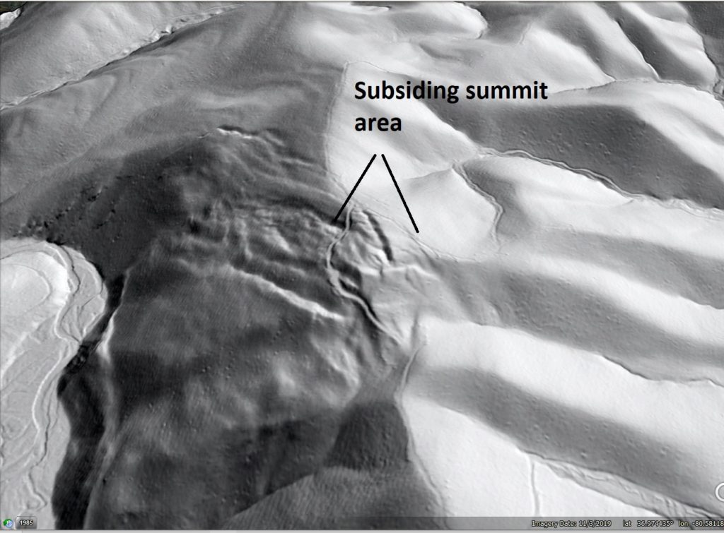
This failure indicates the precarious stability of some rock slopes (particularly dip slopes) in this part of Virginia, even if they host resistant rock types like quartzite. I have hiked along the toe of this feature before, and never knew it was there. The logging road grade along the summit cuts right through numerous scarps. I think this feature is particularly interesting because the headscarps are found on the back side of the ridge crest, meaning the summit of Buck Hollow Ridge has lowered slightly due to the failure.
The slide has developed on a dip slope, with slate/phyllite beds being the likely seat of the basal failure. Dipping quartzite beds nearer the surface are visible in the lidar imagery, as are subtle flatirons within the landscape around the slide. Progressive undercutting of the toe by Big Laurel Creek may have kept this sliding intermittently active for a lengthy period. It makes me wonder what a large-scale, man-made cut along the toe might do…

4. Folded Chilhowee quartzite beds on Poor Mountain, Roanoke County
Poor Mountain is topographically impressive. It absolutely looms above Interstate 81 south of Salem. Despite its size and steepness, its slopes are mostly forested and minimal outcrop is visible. Lidar hillshade imagery shows nice folds in the basal Cambrian/latest PreCambrian Chilhowee quartzite that supports Poor Mountain’s steepness and elevation.
The obvious folds extend about 2,000 ft (600 m) over the land surface in the image above. Their amplitude is exaggerated because they are viewed on a slope and not in a vertical cut, but folding is definitely present. The yellow lines in the image below approximate contours on the land surface, and beds can be seen to cut steeply across contour before paralleling it, and then cutting across it again.
Folding is extensive in the Chilhowee is extensive across the northwest face of the mountain. The lower image below uses lines to call out some of the structures in the foreground.
5. Rock Castle Gorge rockslide, Patrick County
Rock Castle Gorge is actually named for clusters of terminated quartz crystals found in the area, but its Blue Ridge Escarpment location makes it a very rough and rocky place at the larger scale. A main loop hiking trail through the gorge passes through the upper portion of the rockslide shown below, which is conspicuously bouldery and rocky to an observer on the ground.

The still image below shows what I believe to be the route of the hiking trail. I have walked the trail several times, though not for a number of years.
The texture of the slide mass shows the presence of different materials, which are likely schists and amphibolites. The chunky, bouldery material appears to overlie less bouldery material, and is also partly buried by less bouldery material derived from upslope. The bouldery material is clearly derived from the resistant horizon cut by the slide. I have tried to delineate these material-specific zones below.
A visit to this feature would quickly indicate how the stacking order of material in the slide mass reflects position of the in-place materials on the slope. Whether this slide is the result of a single failure or successive failures is unclear. It is also somewhat unique in the area. Despite its steepness and the frequent occurrence of dip slopes, the Blue Ridge Escarpment and its intensely folded metamorphic outcrops seem to host far fewer landslides than the folded/faulted sedimentary Valley and Ridge to the west.
-
Low-displacement landslides explain unusual West Virginia landscape features visible in lidar imagery
by Philip S. Prince
Lidar-derived imagery reveals many fascinating details of Appalachian landscapes, some of which are initially a bit puzzling. Fortunately, if the imagery is sufficiently detailed, it can often provide a rational explanation for the puzzling features. Landslides in the early stages of movement (or slides that have experienced very little movement before becoming dormant) often generate unusual small-scale landforms like the examples in this post. While these features would be noticeable to a geologist on the ground, they are certainly best appreciated (and explained) with the help of 1-meter lidar data! These sites are all located in Randolph County, West Virginia, and would likely be nearly unnoticeable in lower-resolution digital topography data sets.
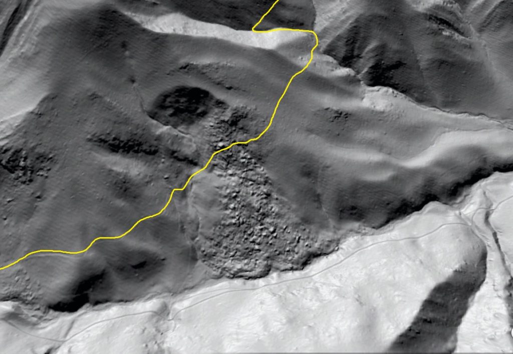
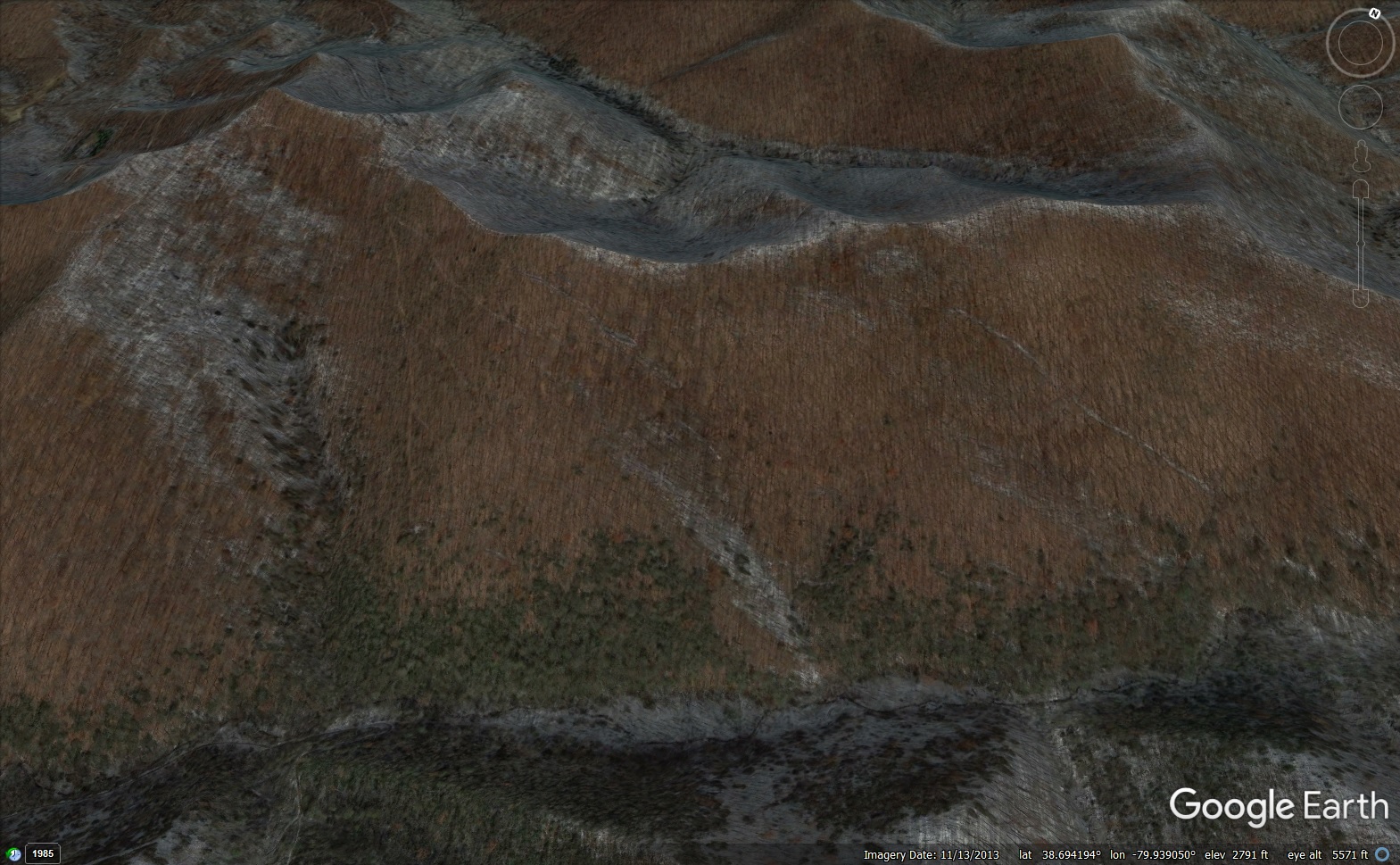
The mountainside shown below hosts several elongated trenches or gashes that are plainly visible in lidar hillshade imagery. A matching air photo image is shown for comparison. The trenches are nearly invisible in the air photo, and while they would be noticeable on the ground, their size (up to 200 ft or 60 m long) and the forest cover would likely obscure their context.
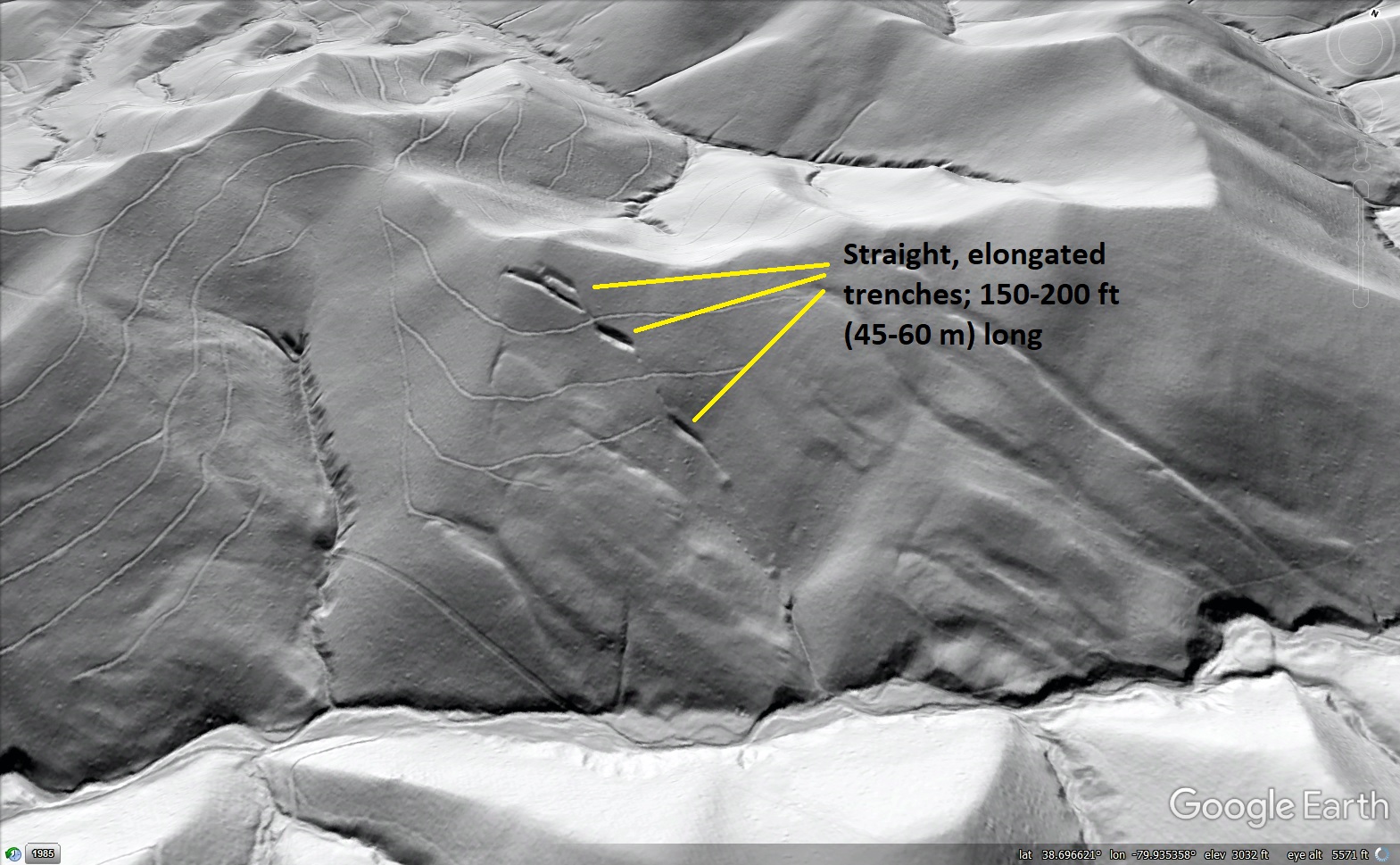
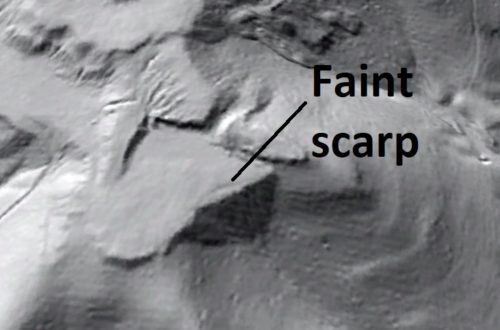
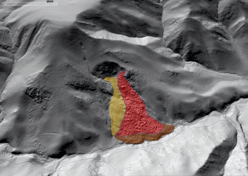
The trenches resemble mining prospects that are common throughout Appalachia, but this zone of Appalachian stratigraphy (Foreknobs Formation; upper Devonian) is not a mineral or coal producer. The trenches also do not cut perpendicular to bedrock strike, a common prospect orientation to expose numerous bedrock units in a single excavation. The trenches don’t follow the typical prospect rules because they are actually small “pull-aparts” along the edges of a large, thin blockslide (a type of landslide defined by a moving, intact mass of stratigraphy). The blockslide has only experienced a very small amount of downslope movement. The first image below shows the entire slide covered by a transparent polygon. The second image points out the laterals (edges) of the slide as well as its toe, whose slight movement has deflected the stream at the base of the slope. The laterals are very subtle and would likely be challenging to identify in the field on the heavily forested slope.
The “pull-aparts” are open gaps between the slide mass and intact slope. They are almost certainly filled with soil and organic debris to some extent, but do not appear to be full grabens, or downthrown blocks, of the slide mass. Presumably, grabens have not formed because the sliding mass is quite thin and the cohesion of the rock composing the sliding layer prevents the gaps’ edges from collapsing. The pull-aparts have formed at stepovers on the left lateral failure surface of the slide, and are thus a result of the shape of the slide mass and its direction of motion.
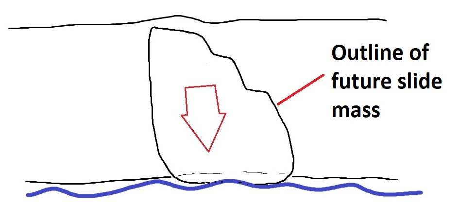
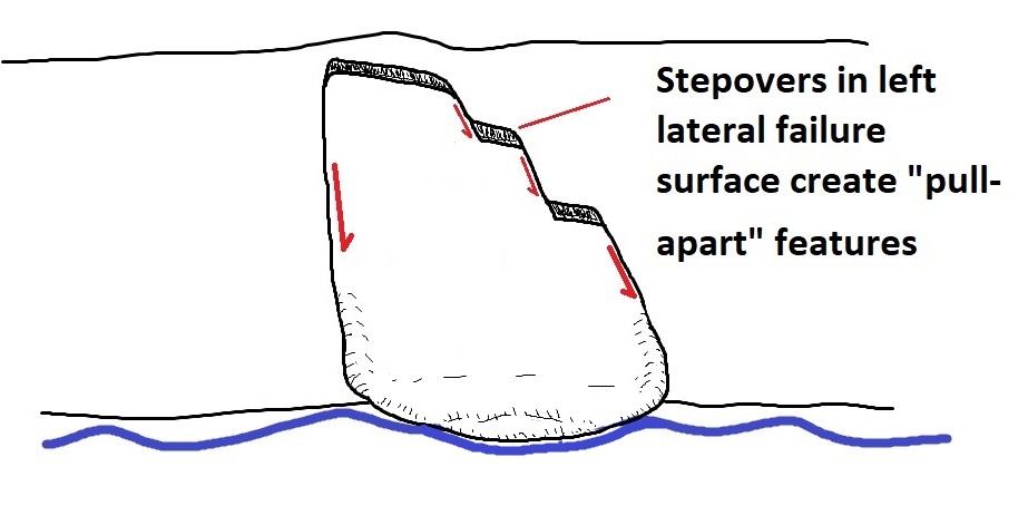
The stepovers and overall angular outline of the slide results from its development within highly jointed or fractured sandstone. As strength of the underlying shale layers is exceeded by the weight and downslope force of the sliding layer(s), the slide mass preferentially disconnects along existing weaknesses in the rock. I have not visited this slide and have no idea of its movement history, but logging roads cutting across it are not disrupted. Material stored in the pull-aparts or in uplifted stream sediments at the toe could provide some insight into when the slide was active.
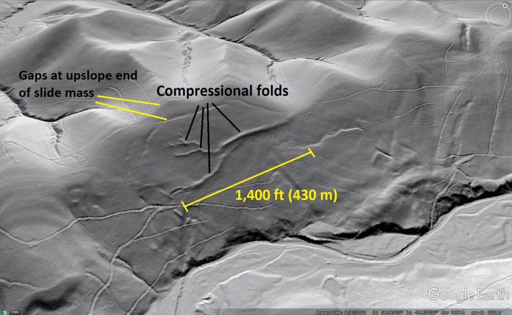
A few miles to the northeast on the same ridge face (and thus the same stratigraphic interval), an unusual vein-like pattern of tiny ridges is visible on the otherwise smooth slope. The “veins” extend 1,400 ft (430 m) along the face of the ridge, and are 40-60 ft (12-18 m) across.
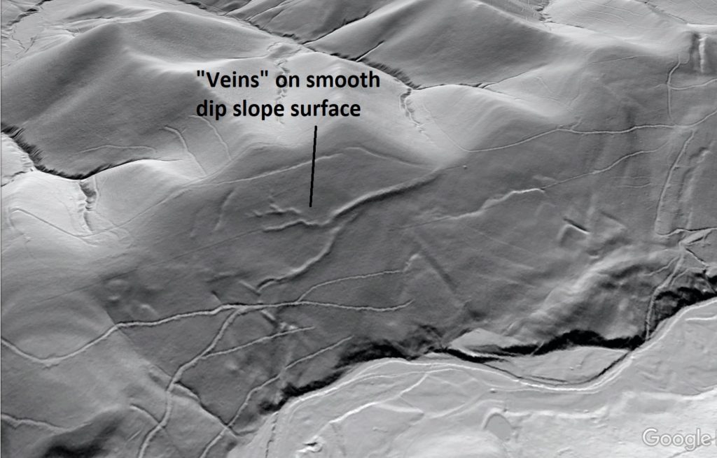
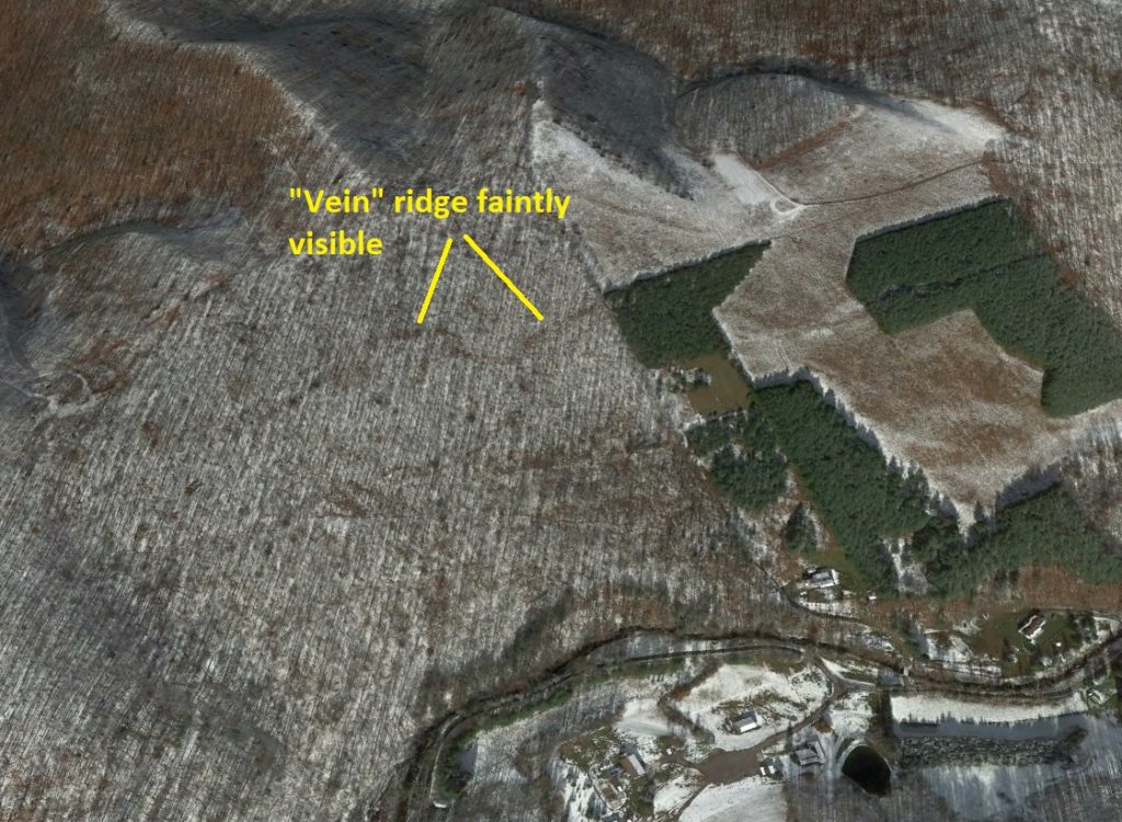
Like the pull-aparts in the previous example, the “vein” ridges would likely be noticeable in the field, but are only faintly visible in the zoomed-in air photo image below.
The “veins” are actually compressional folds developed within a very thin blockslide. Given the width of the veins, the sliding sheet of rock is probably 20-30 feet (6-9 m) thick or so, although this estimate depends of the geometry of the folds. Lidar is again beneficial in interpretation, as it reveals subtle gaps at the upslope end of the slide mass that result from slide movement.

Compressional folding of this type is actually observed in other blockslides in the Appalachian Valley and Ridge, where sliding sandstone layers are so intensely fractured that they can fold at the surface without shattering (see this link). In this Randolph County example, the extremely narrow width of the folds and implied thinness of the slide mass is particularly interesting. The conceptual relationship between fold crest width and the thickness of the slide mass is illustrated below.
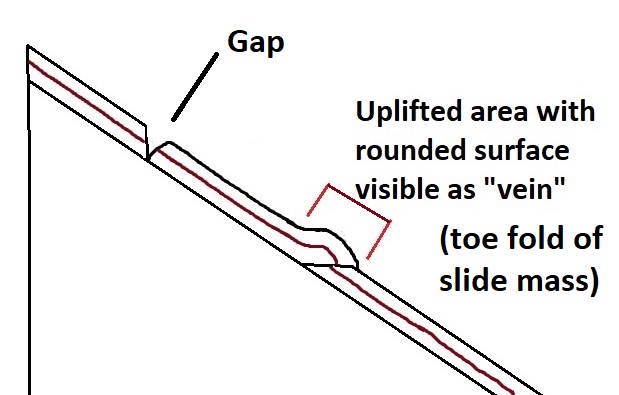
The very basic illustration above shows a simple hanging wall anticline above a thrust ramp at the toe of a blockslide. Many other possible fold and fault related geometries are possible, but almost all involve a fold width notably greater than the thickness of the sliding mass. Given that the slide is 1,400 ft (430 m) across and likely under 40 feet thick, it really is moving like a thin sheet of snow sliding on a windshield as portrayed in the link above. The diagram below is not scaled, but it offers a conceptual view of the slide geometry.
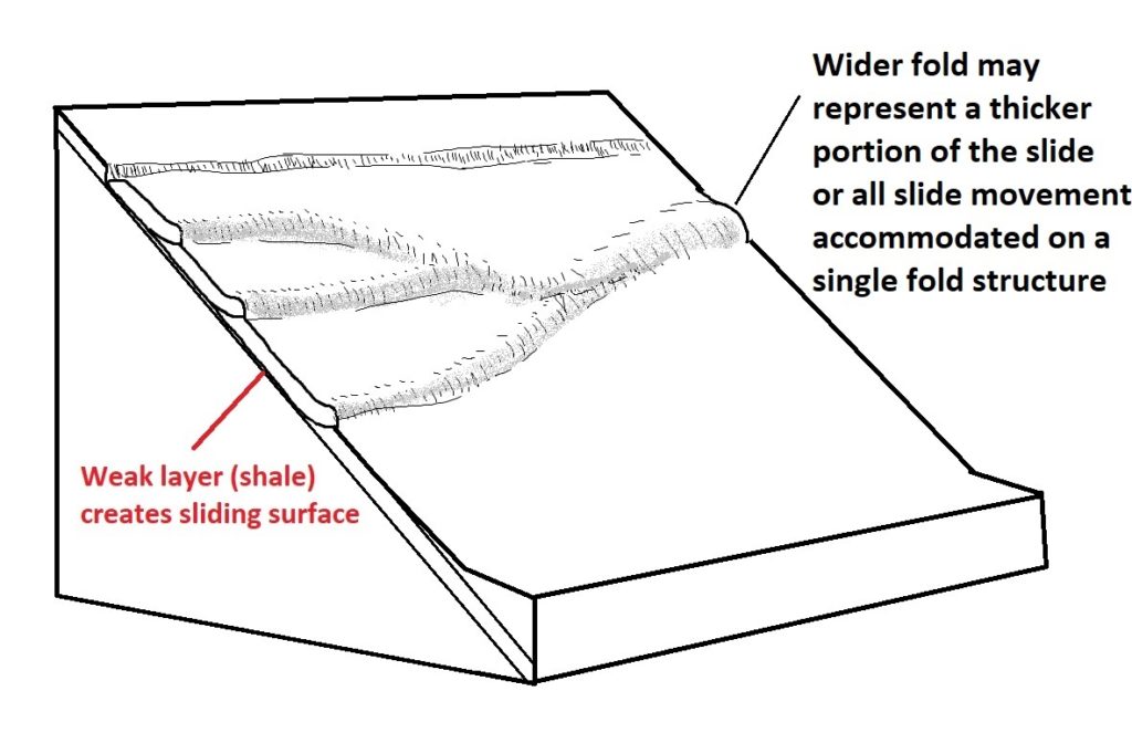
The diagram is broadly based on the three folds visible on the slide, along with the faint upslope gap.
Low-displacement blockslides like these dominate the southeast face of this ridge for about 15 miles (25 km) in Randolph County. While most are limited to the face of the dip slope, some failures are positioned in a way to affect the actual ridge crest, like the slide shown below. In the field, the effects of this slide would be apparent as an elongated depression along the ridge.
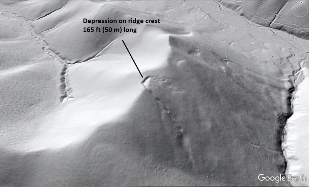
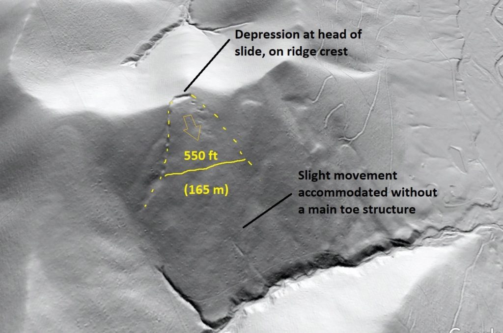
This slide has also experienced only a tiny amount of displacement, allowing the movement to be accommodated downslope without a defined toe.
Like so many older landslides in the Appalachians, the significance and cause of these features is unknown. Because they are so numerous and are only visible using lidar data acquired in 2016, they may represent an untapped resource of useful information about the recent history of Appalachian landscapes.