-
Blowout landslides, part 2: Material movement, and did anything actually “blow out?”
by Philip S. Prince
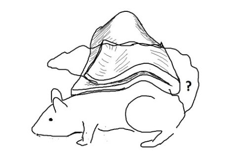
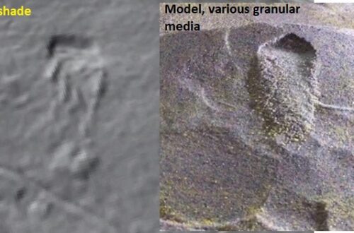
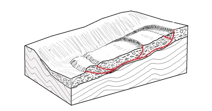
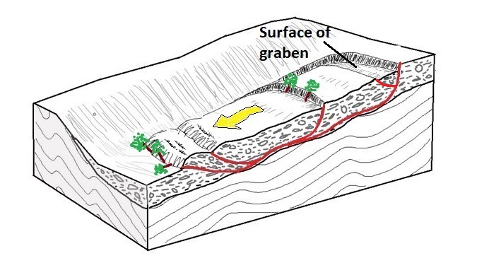
“Blowout” is certainly a peculiar name for a type of slide, but the lidar signature of blowout-type landslides legitimately gives the impression that a force from inside the hillside pushed material out. Observers of these failures developed the same impression, and even a basic physical model (below, right) of this failure style ends up looking like a big hole on a slope that soil spewed out of:
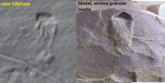
So, what actually happens when these slides occur? I have not personally witnessed one, but I think that a look at details of failure surface shape and the behavior of saturated soil during failure can be used to figure out why blowouts appear to “blow out” instead of just slide. In a second rare move for this page, I again link to an original post on the Appalachian Landslide Consultants site, which presents a host of sketches, a GIF of the model above, and a link to YouTube video of the actual New Zealand slide screenshotted below, which offers insight into the details of blowout material movement. The link can be found at the end of this post.
The most interesting part of this screenshot is the group of small trees being struck by fluidized slide material from the New Zealand failure–specifically the fact that they aren’t being knocked over!
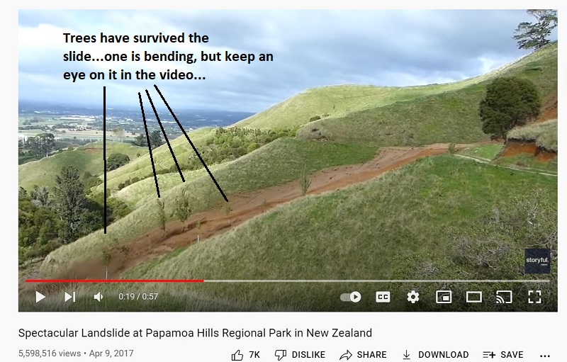
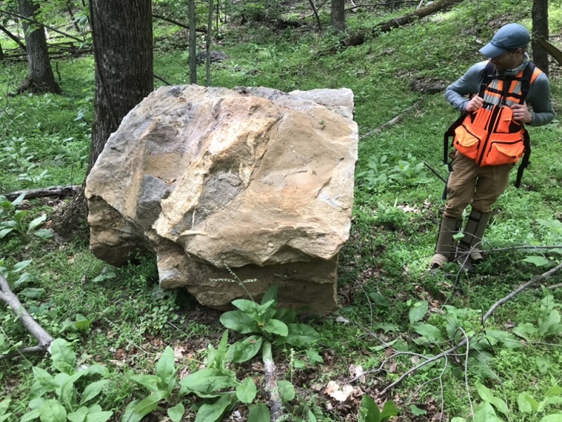
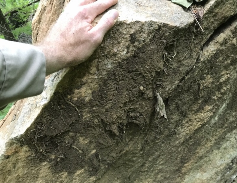
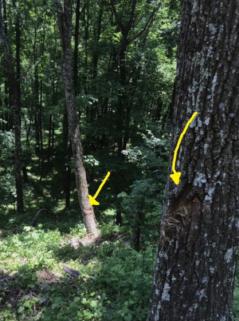
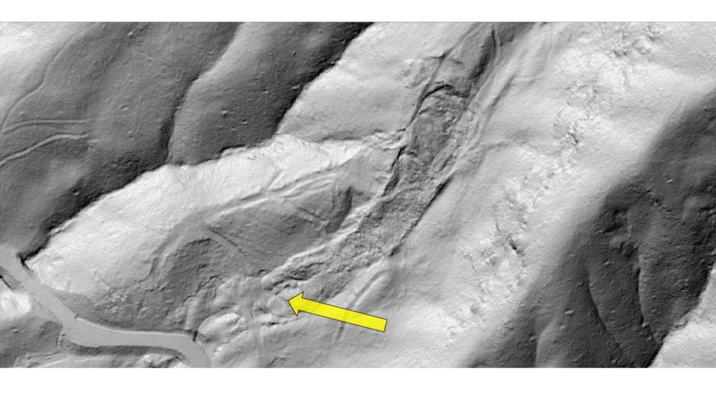
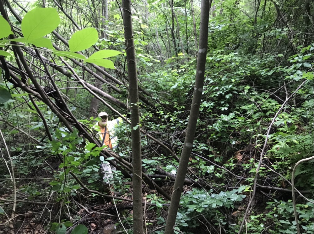
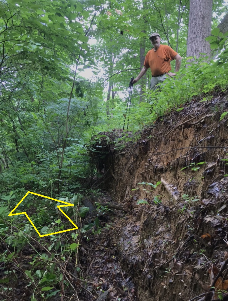
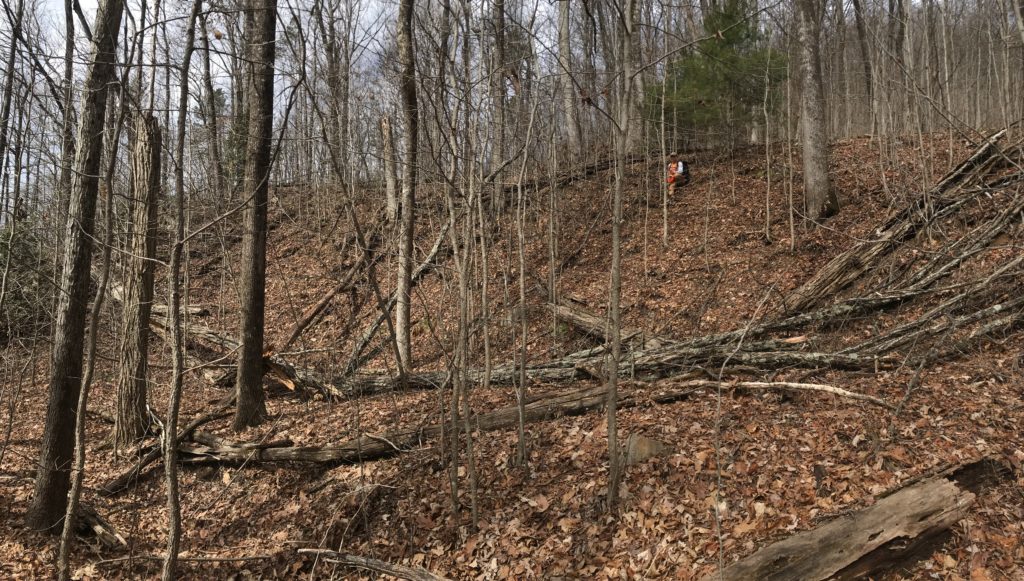
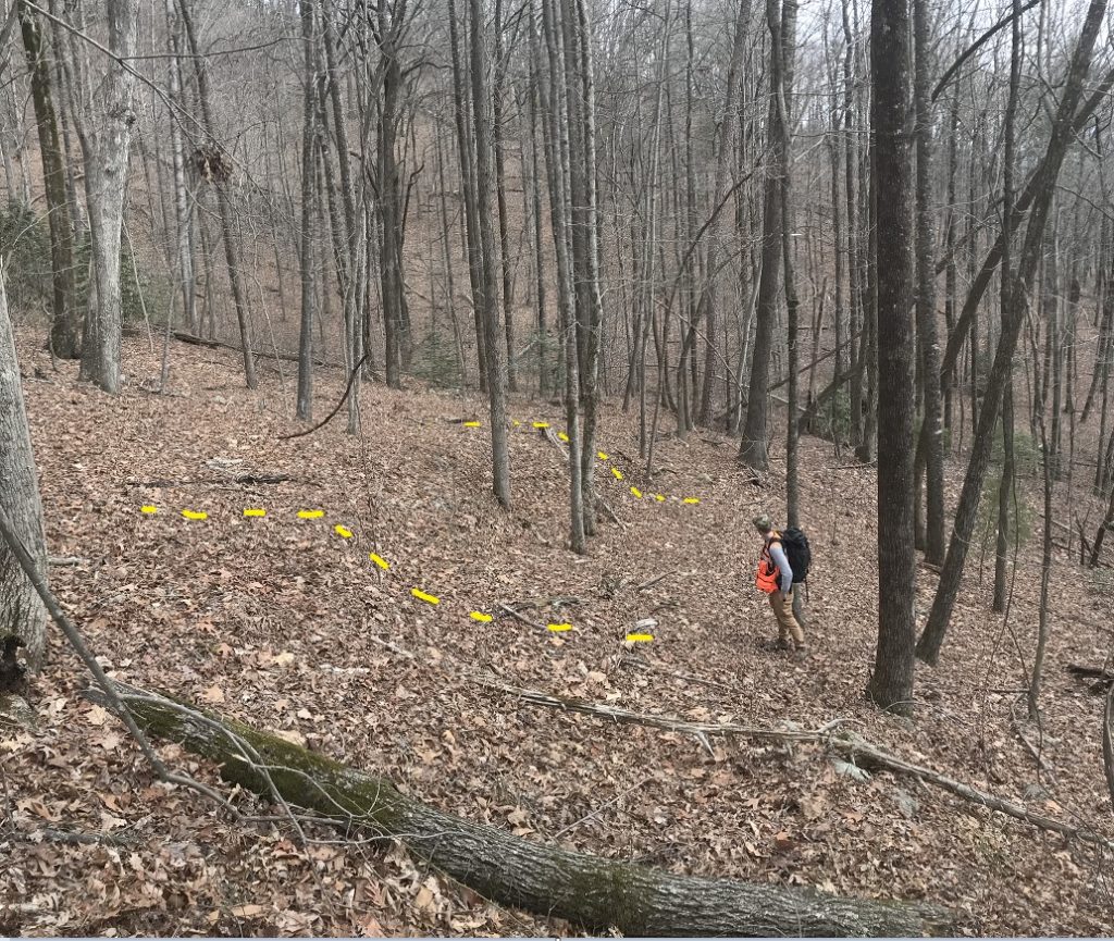
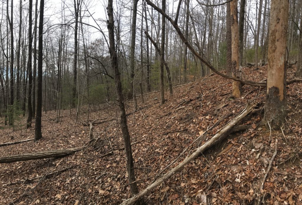
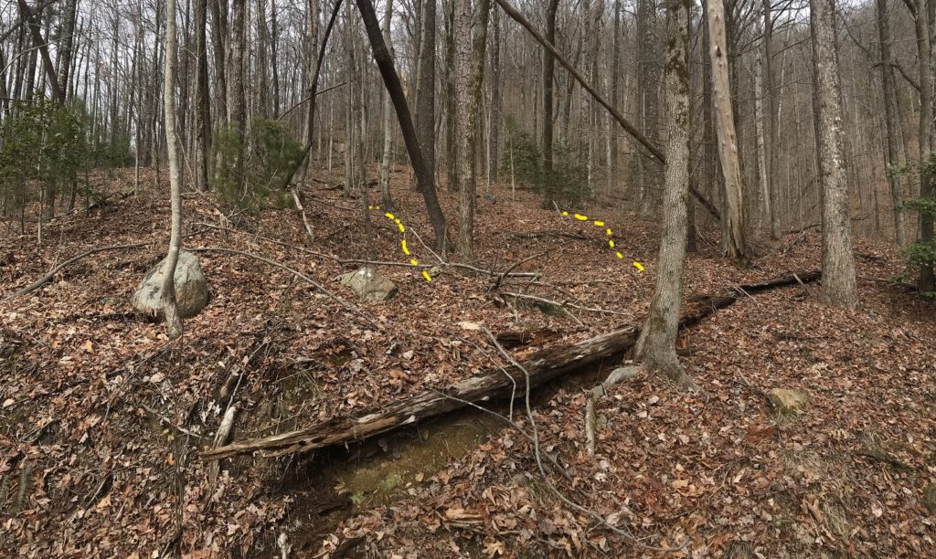
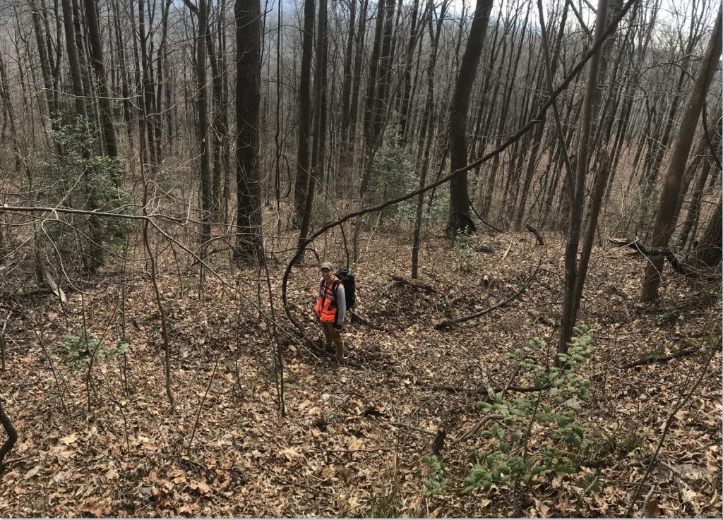
Lack of disturbance of the slopes below blowouts was remarked upon by both Eisenlohr (1952) and Hack and Goodlett (1960), with Hack and Goodlett going to the length of determining just how small of a sapling tree could survive a blowout strike in their study area. I have personally only seen one recent (1 year old) blowout in the field, but it presented the same intriguing lack of slope damage as observed by the earlier authors elsewhere in Appalachia. The photo below shows numerous small saplings killed by the blowout that were not uprooted or even flattened. Most of the tiny trees indicated below are less than 1/2 inch (1.27 cm) in diameter, and while they were damaged sufficiently to be killed, their modest root systems were clearly up to the challenge presented by the blowout material. Their root systems were not even exposed by physical removal of the uppermost soil horizon, which appeared essentially intact. The slide scar is visible in the background.
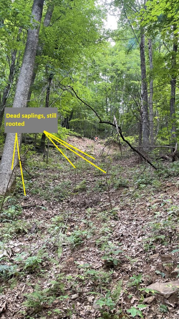
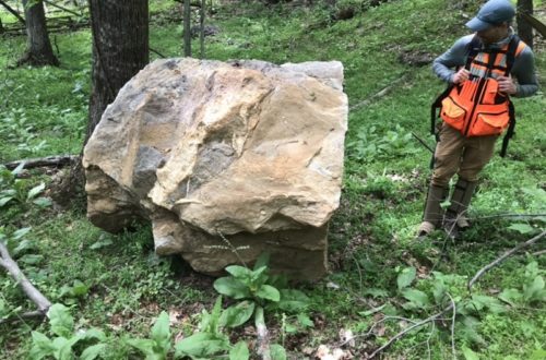
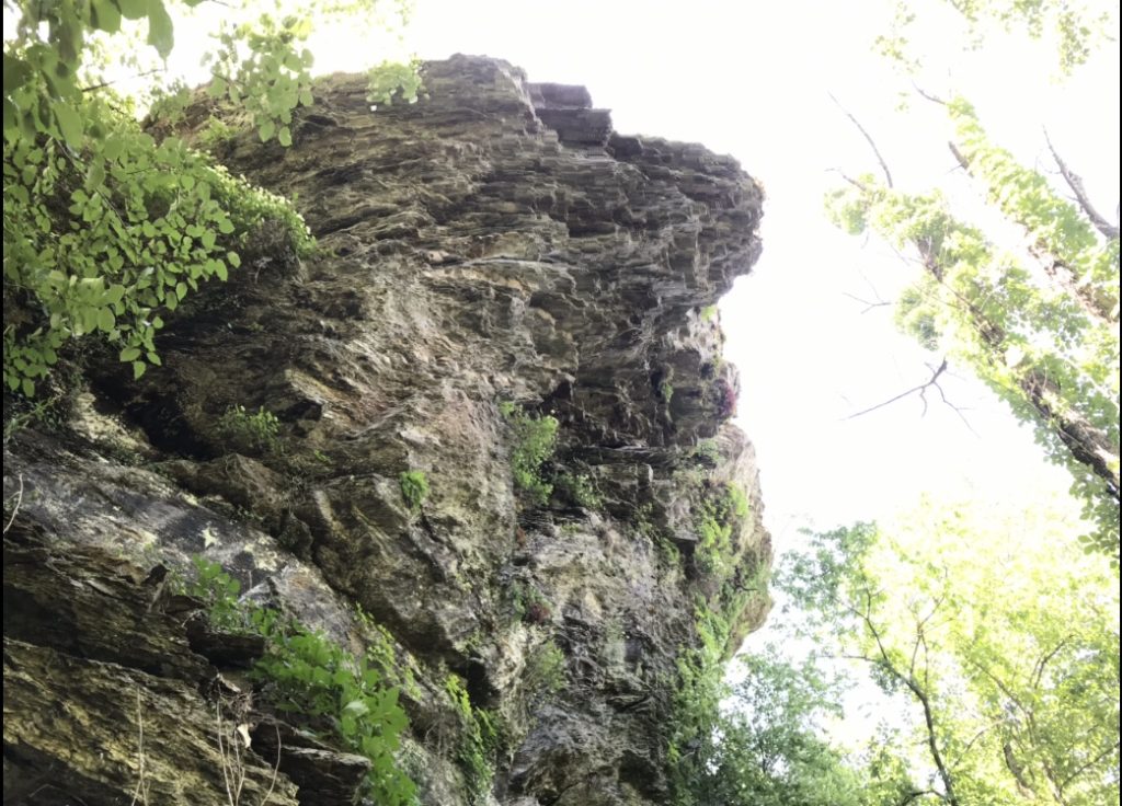
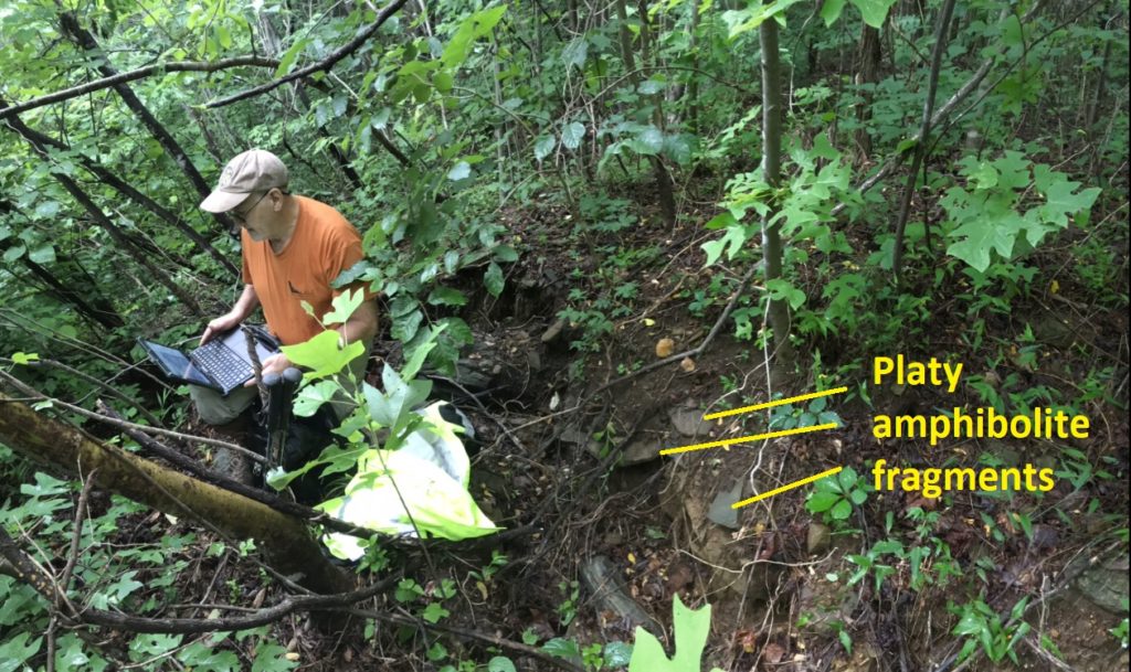
Preservation of small vegetation like this presumably results from extreme fluidization of the sliding–or more appropriately, flowing–mass, which moves like a slurry. Fluid or not, the slide material still contains large clasts, so the little trees presumably avoided these. The image below shows a detail of the colluvium involved in the failure, which exposes the bedrock colluvium contact. Some amount of fill was involved as well; just how much was unclear during this field visit.

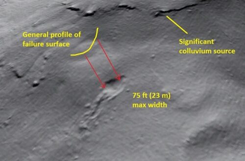
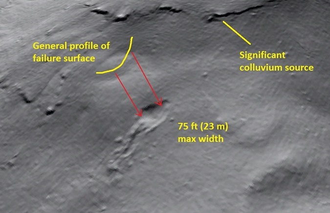
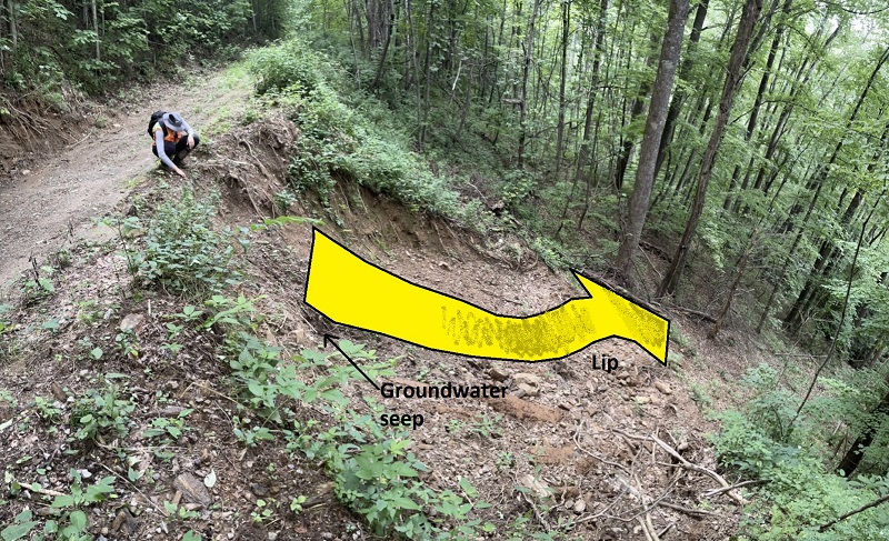
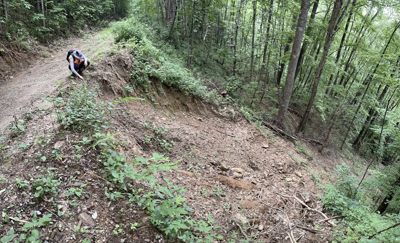
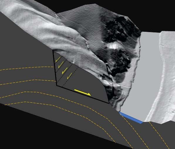
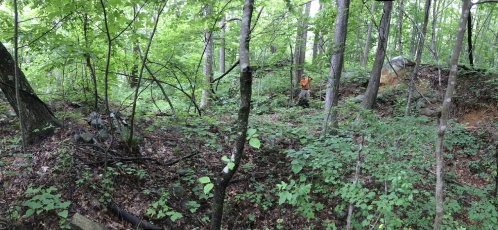
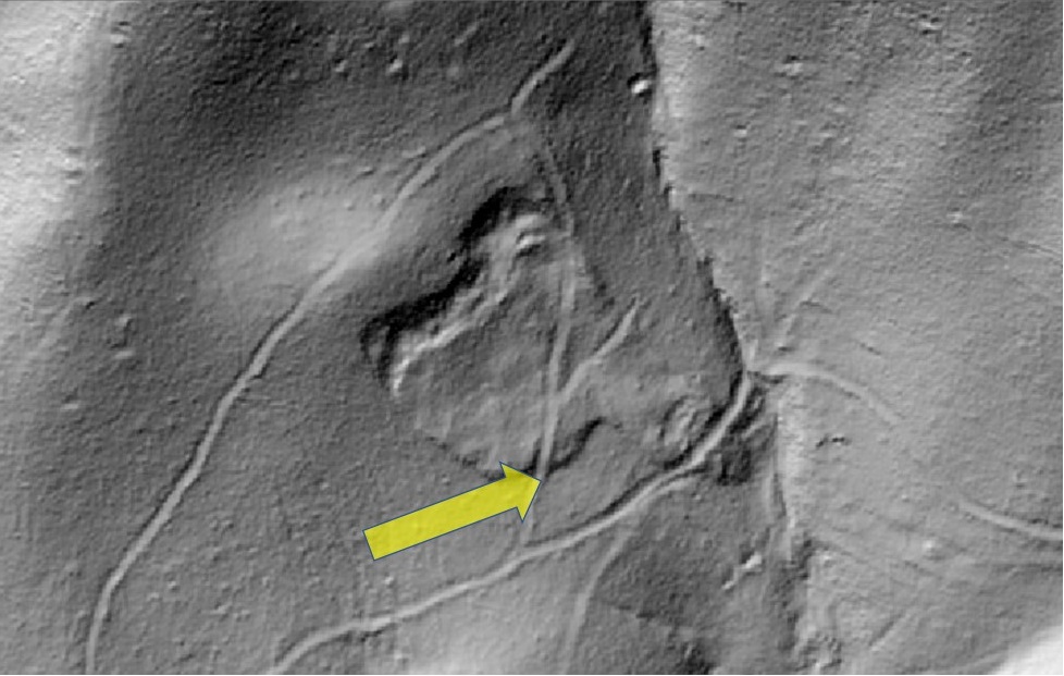
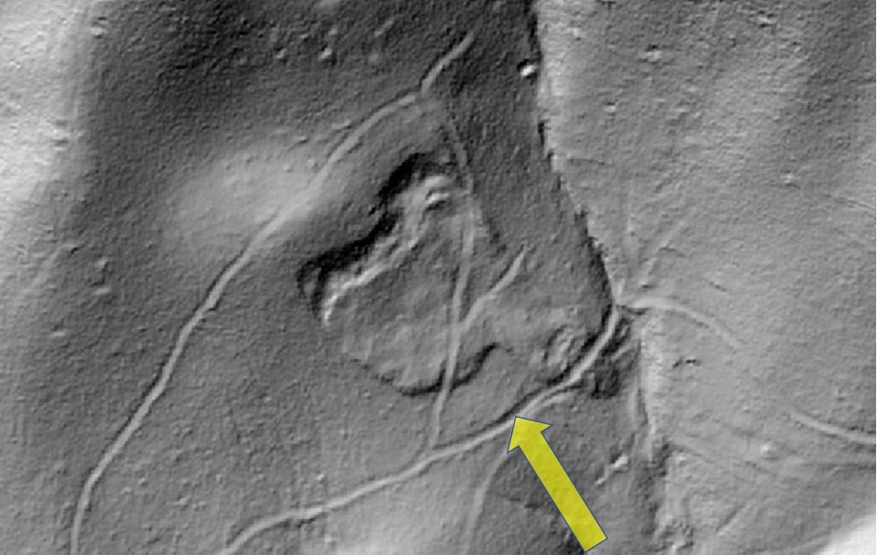
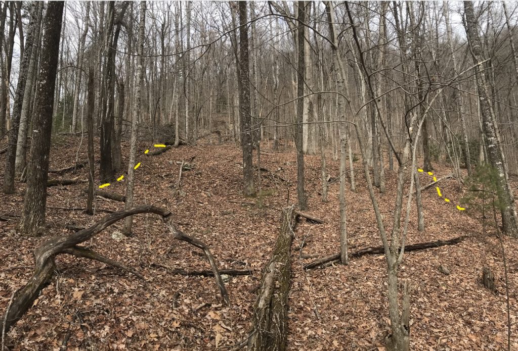
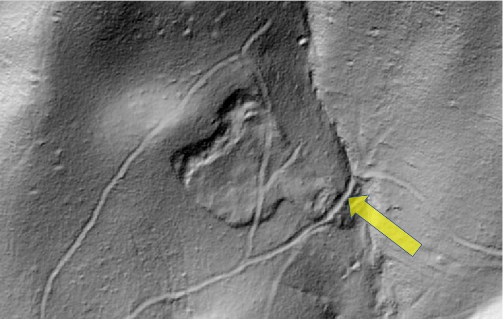
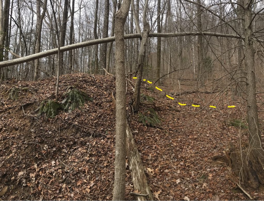
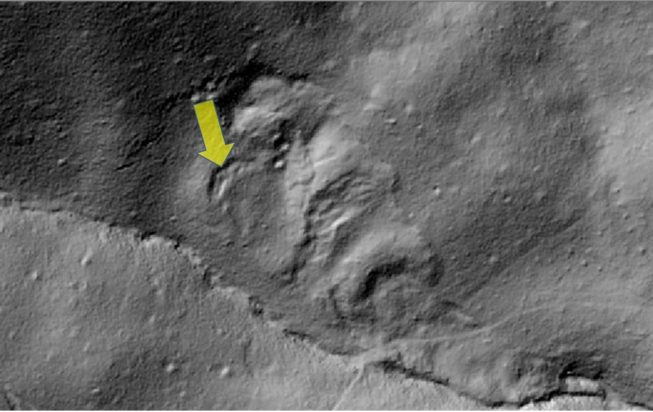
The scar left by this blowout also provides a look at the flat area that creates a lip at the base of blowout failure scars. Rapidly sliding, saturated material obviously moved up and over this lip without degrading it. This path would have caused the material from high in the failure scar to “ramp” out of the scar and fluidize, particularly if it accelerated quickly after initial failure. If observed from downslope, I’m sure this does indeed create the impression of material spewing out of the slope. The images below show the failure scar with and without annotation. Also notable is the seep/wet area, which persists here even in dry weather.
Considering this failure in comparison to the New Zealand failure is interesting, and I presume the degree of fluidization seen in the New Zealand failure likely occurred here to allow preservation of the sapling trunks downslope. Check it all out at the link below.
Link to second blowout post on Appalachian Landslide Consultants, PLLC page
-
“Blowout” landslides and the lidar signature of extreme Appalachian rainfall events
by Philip S. Prince
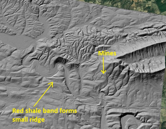
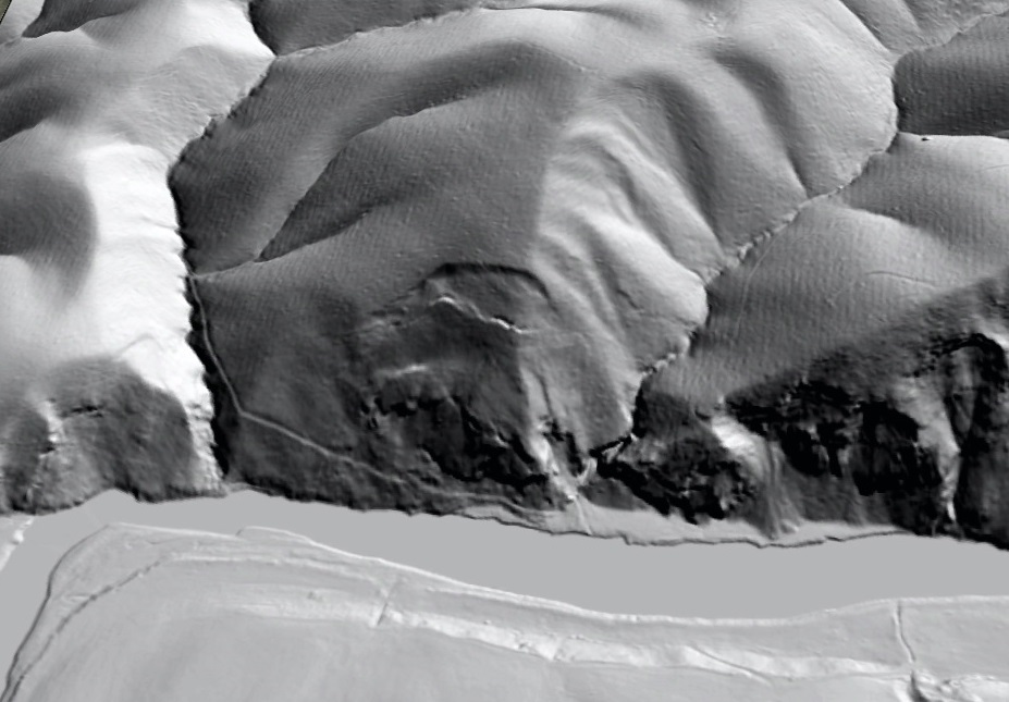
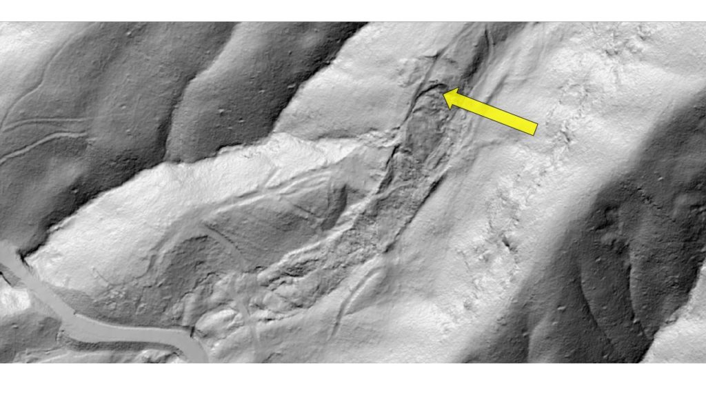
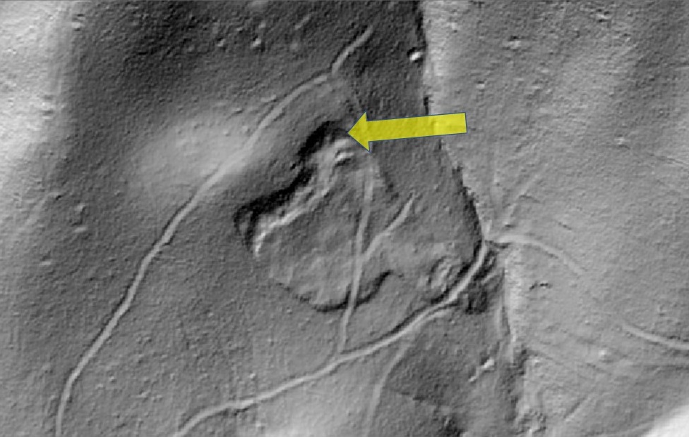
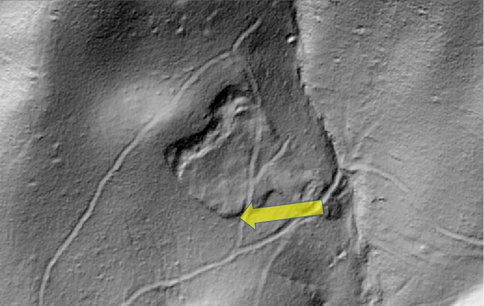
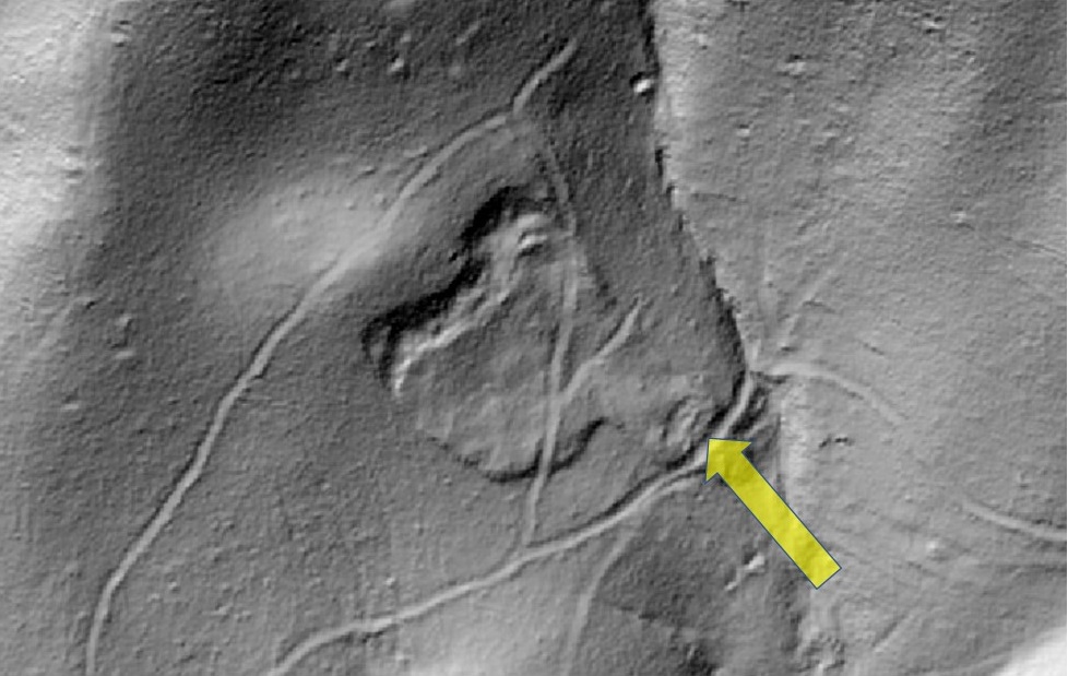
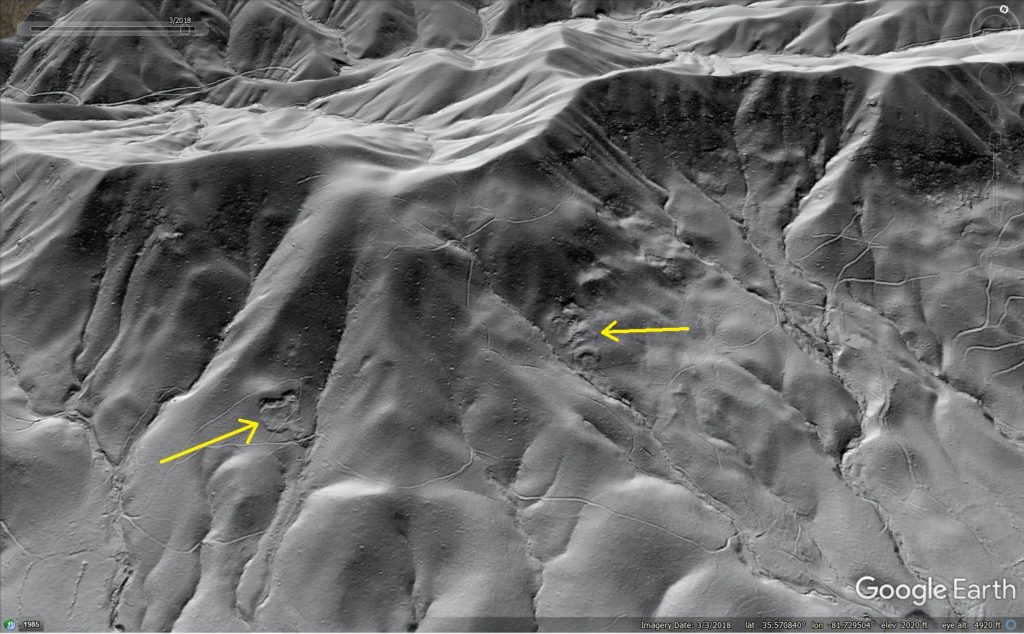
On the night of June 27, 1995, the Albemarle County, Virginia, mountainside shown below received an exceptional amount of rainfall. No one knows how much, but a nearby rain gage recorded ~ 11 inches (28 cm) of rainfall with only 2 hours…the rain event continued for several more hours. Unsurprisingly, a tremendous number of landslides resulted. The slides are clearly visible in this lidar hillshade image, and those marked with yellow arrows are of particular interest in the context of the storm’s outrageous precipitation rate and total, which likely reached 30 inches (76 cm).
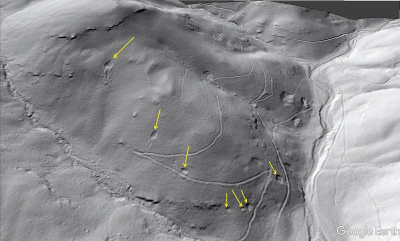
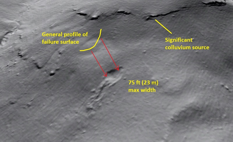
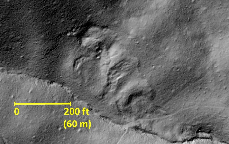
The slides highlighted by the yellow arrows are examples of what William Eisenlohr, Jr., called “blowouts” following a July 1942 storm that produced similar features near Port Allegany and Smethport, Pennyslvania, as a result of similar rainfall rates and totals. Below, a detail of the slide at upper left in the image above shows particular details of the type of failure that inspired the unusual “blowout” name: a curved failure surface and arcuate scar, no erosive track, no intact slide block, and debris spread as a sheet over the slope below. Notably, much debris is missing; the deposit visible below certainly doesn’t account for the volume removed from the scar.
These “blowouts” and their association with extreme Appalachian rainfall events (more than 10 inches (25.4 cm) in under 10 hours) offer up an interesting story about hillslope response to extreme rainfall and the very 21st century ability to see that response with 1 meter (or better) resolution lidar. Linked below is a full-length post I recently wrote about these slides on the Appalachian Landslide Consultants, PLLC, page, which shows blowouts related to atypical storms in several Appalachian settings:
Link to original Appalachian Landslide Consultants post
I usually don’t base a post on this site about external material, but in this case pasting a link is admittedly more appealing than re-posting all the figures and text. The Appalachian Landslide Consultants page also allows images to expanded to full screen with a click, which is a plus. Original reports about the slide events are linked in the full-length writeup, and I personally enjoyed checking out the sites highlighted in Eisenlohr (1952) and Hack and Goodlett (1960) (shown below) with 2017 lidar!
-
The waddling boulder…a storm-induced trundle* event?
by Philip S. Prince
*yes, trundle will be defined at the end.
I see lots of boulders in the course of my fieldwork, but this one just looked different…
Appalachian Landslide Consultants geologist Aras Mann (pictured above) and I spent a fair amount of time trying to figure out just what made this boulder look so strange. We first noticed its apparently soil-stained color, unusual in its rainy Rutherford County, North Carolina, setting. The boulder also had mud and dead vegetation caked on its corners and edges.
Eventually, we looked towards the slope behind the boulder’s resting place and noticed two flattened saplings and alternating, diagonal gouges in the soil (yellow arrows below) leading down to the boulder. These details made it clear that the boulder had recently rolled into place.
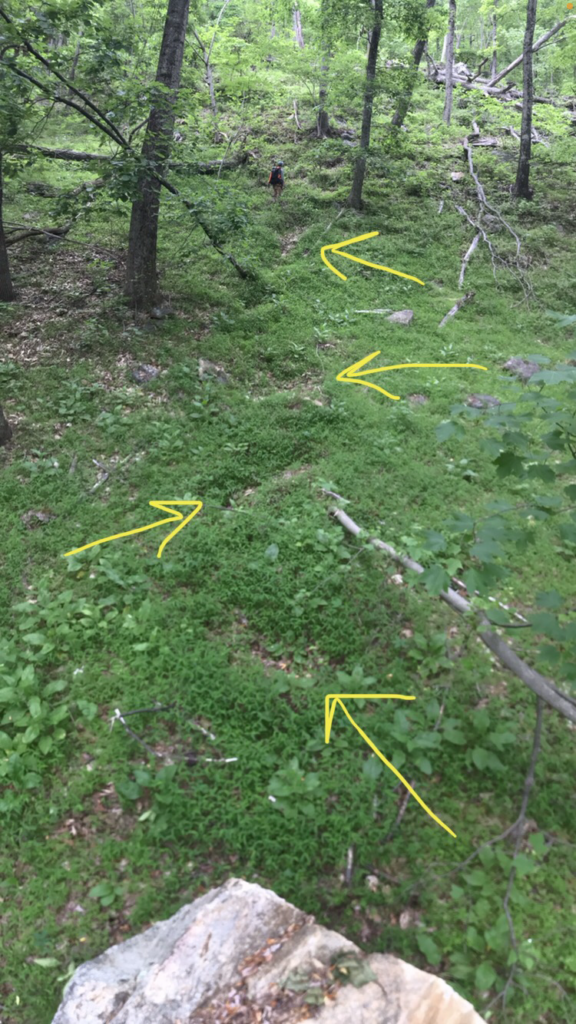
This was (and remains) the first and only boulder I have personally seen that has rolled or tumbled and come to rest recently enough for its track to be visible in the field. I thought the diagonal gouge marks were particularly interesting. For whatever reason, they caused me to visualize a slow, “waddling” rolling style like that of an American football or rugby ball rolling downhill. The boulder had not traveled particularly far across the flat area where it came to rest, and I thought the “waddling” style might explain this.
The boulder had, however, traveled down a significant slope prior to reaching the flat, and should have been moving at good speed. I could not really make sense of the gouge marks, travel distance, and steep slope origin. When I can’t visualize structural geology scenarios, I turn to sandbox models. I tried to do the same here, and I was easily able to produce alternating diagonal “zig-zag” rolling tracks with model boulders and a sand tray.
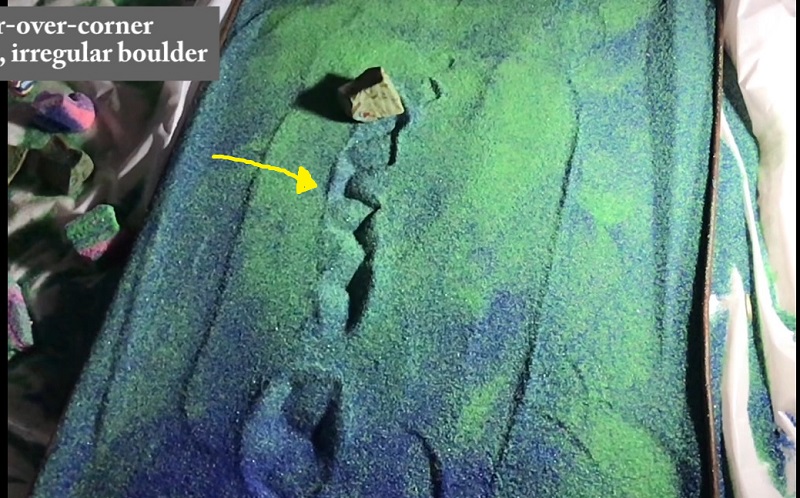
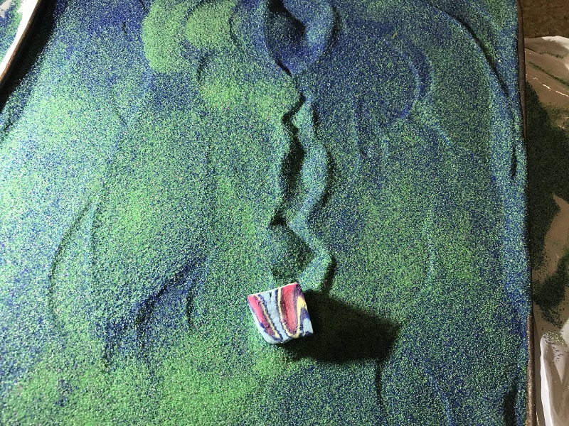
My model boulders were made of dried play-doh, which had been cut into shapes reminiscent of the recently emplaced Rutherford County boulder. I let these roll down a tilted strip of carpet, which caused them to tumble as they accelerated before rolling out across the nearly flat sand tray surface. Tumbling the model boulders turned out to be rather interesting, and was sort of like shooting dice for people that like geology and interesting visual patterns. To summarize the results of dozens of rolls, the model boulders produced either zig-zag tracks from corner-over-corner rolling or longer tracks with a helical pattern from face-over-face rolling. These rolling styles and the resulting tracks are shown in the video linked below (a helical, edge-over-edge pattern is shown in the link image).
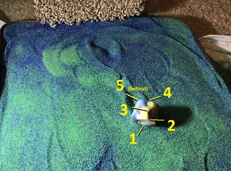
Corner-over-corner rolling occurred when the model boulder did not tumble smoothly down the carpet and thus did not reach a high speed. Once a corner-over-corner roller hit the sand tray, it seemed to lose energy more quickly than the face-over-face rollers, presumably due to the deep gouging of the edges and greater length of the boulder’s diagonal. The image below shows the sequence in which the edges and corners impacted the sand to produce the zig-zag pattern.
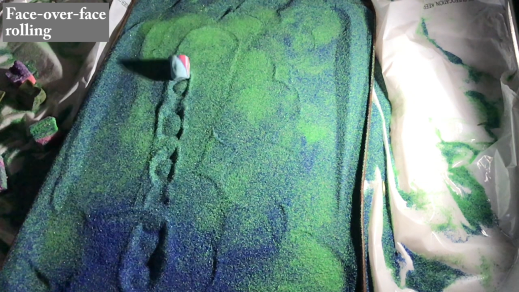
Regular, face-over-face tumbling down the carpet allowed the boulders to reach higher speeds and travel notably farther across the sand tray. The helical pattern (below) results from a slight irregularity in the model boulder’s rectangular prism shape; one edge was slightly rounded.
The models made it clear that the real boulder probably did not make any sort of unusual “waddling” rolling style. Its shape, combined with corner-over-corner tumbling, would have allowed it to make the zig-zag, diagonal gouge marks in its track while rolling in a generally straight line at moderate speed. The corner-over-corner style is a less efficient and sort of off-axis style of movement, but I imagine that to an observer, the boulder would have appeared to simply be rolling at the time of its emplacement.
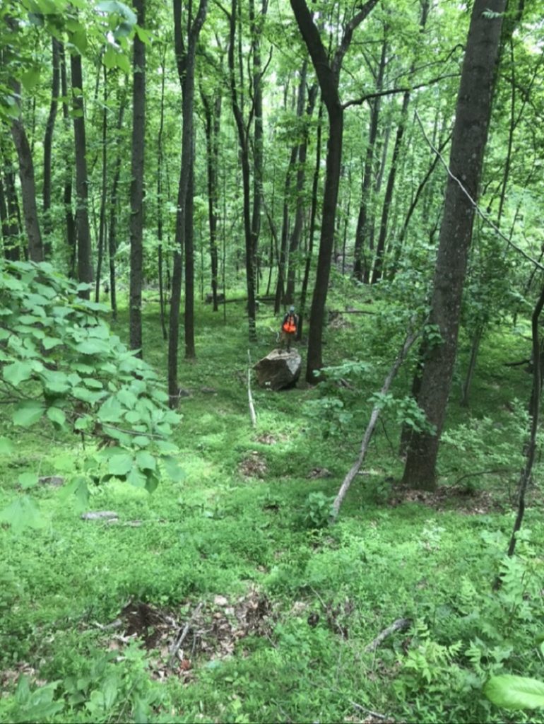
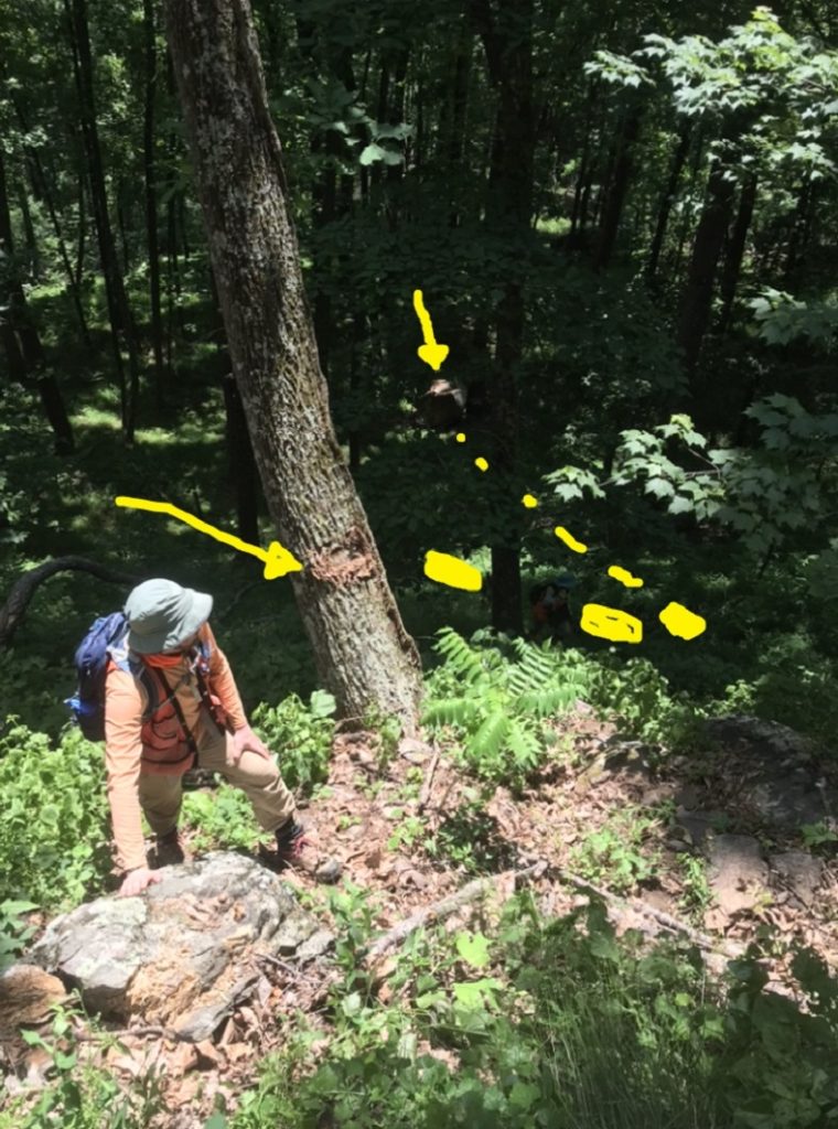
On a later visit to this site, we tried to find the boulder’s place of origin on the slope. The boulder’s track could not easily be traced by impact marks on the slope surface, but scarring on tree trunks made its path quite clear. Corey Scheip (BGC Engineering) examines one of the tree scars in the image below. The dash marks generally show the boulder’s path after the tree impact. It was deflected to the right before continuing downhill to its resting place, shown with an arrow in the darker portion of the image.
The boulder hit several trees on its way down, all of which bore similar scars. The trees were offset in their locations, suggesting the boulder deflected from one to another and followed a Plinko-style path down the slope. The lack of a straight path obviously limited the boulder’s speed and may have prevented it from attaining a faster, face-over-face tumble.
So, where does “trundle” figure into all of this? When I searched YouTube for videos of rolling boulders to try to better understand the origin of the diagonal gouge marks, I repeatedly found “boulder trundle” videos. Apparently, “trundling” is the act of purposely rolling boulders down slopes, often by prying them loose with levers. Limited field evidence still visible during our second visit to the site suggested that the recently emplaced boulder had started rolling after it was pried loose or struck by a falling tree. A tropical depression had passed through the area several months prior, and high winds along steep slopes had knocked down numerous very large oaks. The boulder’s tree scarring and faint slope track appeared to begin just below the base of one such felled oak, suggesting the rolling of the boulder was indeed a natural, storm-induced “trundle.” I’m not sure how often tree fall triggers rockfall in this region or elsewhere, but this scenario has certainly added another element to my own evaluation of possible slope hazards.
-
Two mappings of a folded thrust fault in the Appalachian Valley and Ridge, 100 years apart
by Philip S. Prince
Well, actually 98 years, but close enough…
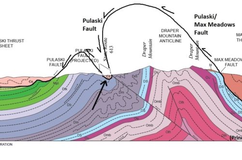
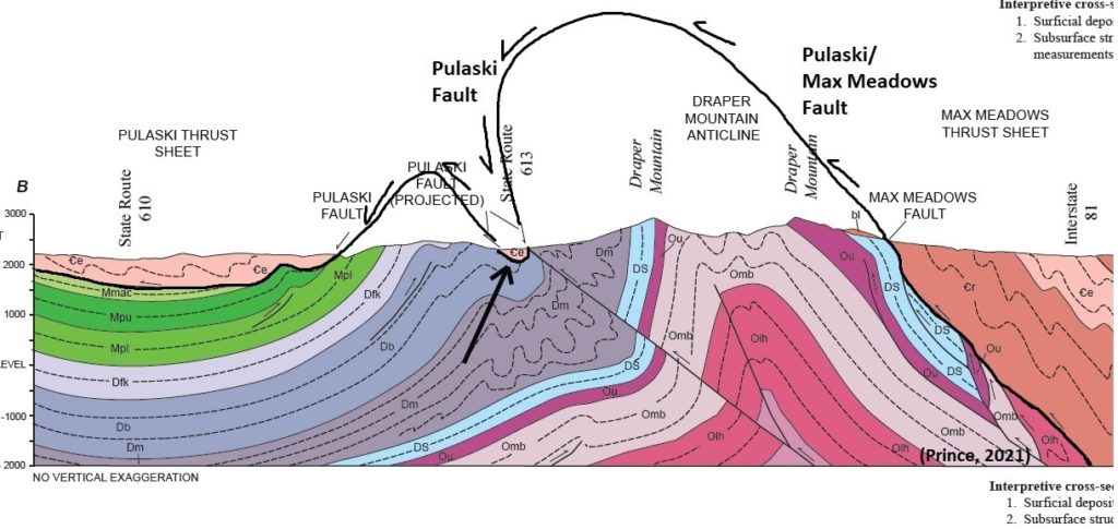
Northwest of Hamilton Knob in Wythe County, Virginia, two narrow outcrop bands of Cambrian dolomite are entirely surrounded by Devonian-aged shales and sandstones. These dolomite bodies are tiny klippen that are separated from the Devonian units by the Pulaski Thrust Fault, which has been folded into two anticlines separated by a narrow syncline in which the klippen occur. I mapped in this area during the last year and a half, and I think this might be the most extreme example of folding of the Pulaski Fault system within the Valley and Ridge. In the cross section below, the large black arrow points to one of the klippen. The curving black line is a projected estimate of the folded geometry of the Pulaski Fault prior to erosion to present-day levels.
The GIF below shows the approximate line of section above and points out two of the “micro-klippen.” The klippe crossed by the section line is just large enough to impact land use, allowing it to be seen as a brown, cleared area surrounded by the forested, acidic Devonian shale/sandstone landscape. The smaller klippe is too small to impact vegetation or land use.
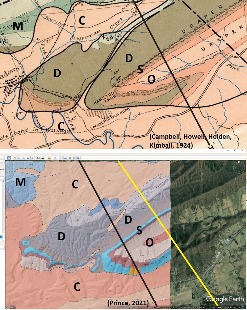
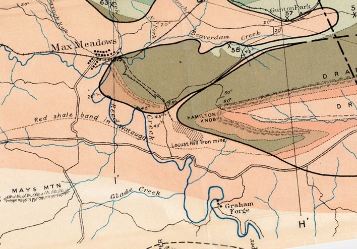
These klippen are made even more interesting by the fact that they were mapped and correctly interpreted in 1924! The image below compares a 1924 map by Campbell, Howell, Holden, and Kimball to my 2021 mapping, which was produced entirely through new fieldwork and lidar analysis. M, D, S, O, and C denote Mississippian, Devonian, Silurian, Ordovician, and Cambrian outcrop zones, respectively. The curving black lines in the 1924 map are the Pulaski Thrust, which correctly encloses a narrow sliver of Cambrian rock (peach) between two extensive Devonian (dark green) outcrop fields (south of “Creek” in the Beaverdam Creek label and the 45 dip measurement). Comparing these maps separated by 98 years and considerable changes in land use, geologic exposure, tectonic understanding, and imaging technology is very interesting to me. The same patterns and structural relationships are obviously present in both to a high level of detail, which is impressive given the much larger scale of the 1924 map project. The map is part of a massive, regional overview of coal resources in the Virginia Valley and Ridge, which is why I never took the time to check it out until now. This “Valley Coalfield” report is linked here; the map comes at the very end of the 381-page document.
Identification and mapping of the distinct rock in the klippen in 1924 is not terribly surprising. Due to land use at the time, vegetative cover was much less extensive and outcrop was more visible. Iron ore also occurs along carbonate-Devonian shale contacts in the area, so special attention was paid when those rock types were expected in an area. The interpretation of the klippe as the result of folding of a thrust fault, however, is quite interesting in light of understanding (or lack thereof) of fold-thrust belts at the time. I am impressed that this intensely folded thrust model arose out of the prevailing theories about the nature of thrust faulting at the time, but it provides just about the only way to explain the architecture of the rocks in the area. The cross sections below compare the 1924 interpretation (line of section is the straight black line in the 1924 map) with my 2021 interpretation, with colors adjusted to match. The 1924 section was developed slightly north of mine, but the overall context of the klippe related to adjacent fold structures is the same. Black arrows point out the Cambrian micro-klippe in each section.
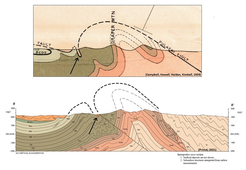
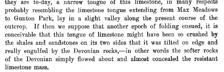
In 1924 and today, a key component of understanding these micro-klippen is explaining the tightness of the syncline that preserves them. After my work in the area, I think it is largely attributable to mechanical contrasts in the rock mass. The dark green horizons in the sections above are shale-rich and weak compared to the overlying light green Mississippian sandstones and underlying Siluro-Devonian sandstones (light brown). The base of the Pulaski Thrust Sheet itself (pale orange) is probably mechanically weak as well, consisting of thin-bedded carbonate which is often extensively brecciated. As a result, the forelimb of the overall Draper Mountain anticline was able to tightly buckle and nearly enclose a tiny pod of the Pulaski Sheet carbonates. This behavior would not have occurred with a different mechanical combination of strata. Campbell et al. had a generally similar idea, and explain the concept very nicely in pages 83-84 of the Valley Coalfield text. “Engulf” is indeed a nice word to describe their model.
I used the conceptual model below (it’s a very slow moving GIF…wait for it) for my own explanation of the micro-klippen. Early broad folding of the Pulaski and Max Meadows Thrust Sheets occurs when the Draper Block moves onto an underlying flat, probably developed in middle Devonian shale. The future micro-klippen are rotated forward on the forelimb of the block. In this geometry, weak units on both limbs of the Draper Block are poised to slip on or close to bedding planes, setting the stage for a localized “pop-down” syncline in the zone of weak, shale-rich interbeds. This model requires relatively little displacement on the out-of-sequence faults due to the pre-existing ramp anticline geometry, as well as the position of the future micro-klippen on the upper Devonian-Mississippian ramp. Interestingly, Campbell et al. draw the klippen in this ramp position as well, suggesting we placed formation boundaries on similar marker beds.
So, has re-mapping this area offered any improvement on a such a good but 98-year old product? Yes. New mapping is spatially much better; the 1924 map cannot be draped onto an existing surface map with decent accuracy. Subsurface interpretations are also better, applying more rigorous geometric controls obtained by outcrop mapping and detailed lidar topography. Details of the Pulaski Thrust Sheet and particularly its immediate footwall are also better in the newer map, due to its smaller spatial scale and (again) the ability to track individual beds using lidar. The present map results also have much more context within the overall study of fold-thrust belt evolution, both in the Appalachians and in other systems around the world. Even so, the 1924 product is surprisingly high-quality and interpretively ahead of its time. I will actually be using it in my current mapping to the north of this area, as it shows in great detail where coal beds are cut of by thrust faults that are extremely difficult to identify in the field or with lidar.
Beyond the scientific details, I like the 1924 map because its details capture specific challenges of working in the area that persist today. My favorite is marking of the “Red shale band in Watauga” with a dashed line, running just left of, then below, the center of the 1924 map image below. The Watauga Formation, today known as the Rome Formation, is intensely folded and stratigraphically baffling in this area. Determining whether you are mapping near its base or top feels impossible, as marker beds are few and far between. Campbell and his associates obviously jumped on the red shale band in hopes of using it as some sort of recognizable frame of reference within the confusing sea of folds. I did exactly the same thing, as the red shale band is very recognizable in lidar-derived imagery as well as in the field (lower image). It can be tracked over significant distances and does indeed highlight some larger folds within the Rome Formation, some of which help define contacts with the overlying Elbrook Formation as we map it today.
-
Is this the steepest river in the Appalachian Mountains?
by Philip S. Prince
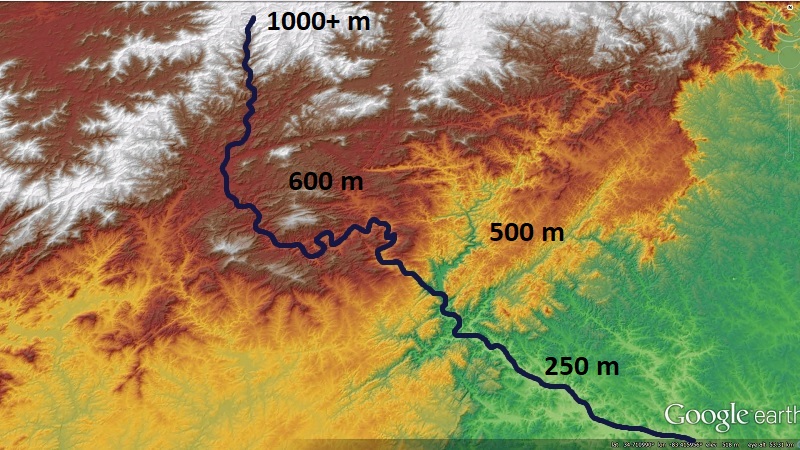
Topographic superlatives are almost always a bit arbitrary, and comparing river steepness is about as arbitrary as it gets. How long of a stretch of river needs to be considered? How big does a stream need to be in order to be considered a “river?” Since a vertical waterfall is the maximum steepness possible, is the biggest river with a freefalling waterfall the winner? How tall does the waterfall have to be? These questions all have merit, and each one can steer this search in a slightly different direction. One reach of Appalachian river, however, stands out no matter which of these parameters is applied: the gorge section of the Tallulah River of northeast Georgia.
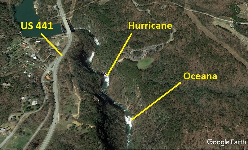
At the upper end of Tallulah Gorge, the Tallulah River drops about 400 ft (120 m) in 1 mile (1.6 km) or so (some sources say 500 ft over this distance). Much of this descent occurs across four huge waterfalls, which are easily visible in Google Earth…and which seem precariously close to US Highway 441. Oceana is the only falls directly accessible to hikers and, in April and November of each year, to whitewater paddlers. Hikers can cross a bridge over the top of Hurricane and approach its base, but the upper two falls can only be experienced from a distance due to their extreme ruggedness. Vertical rock walls are present in much of the upper gorge.
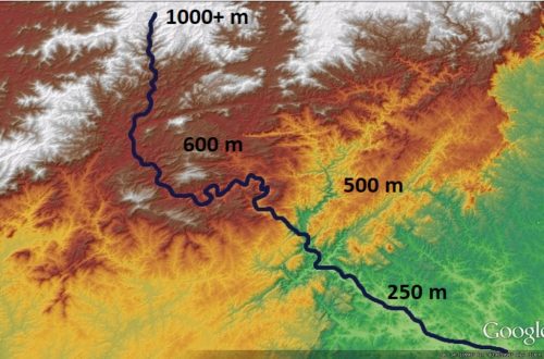
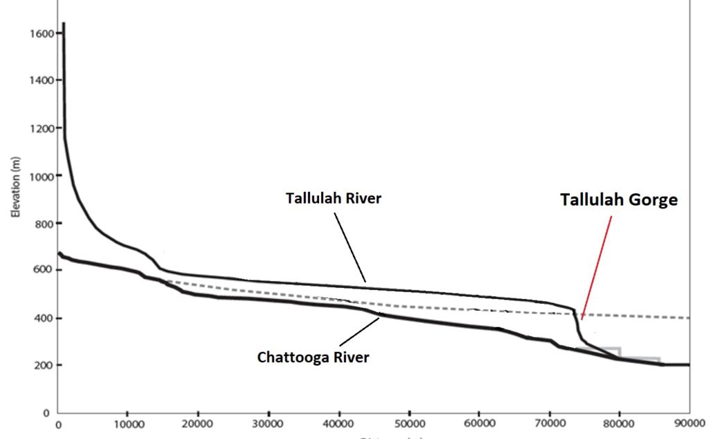
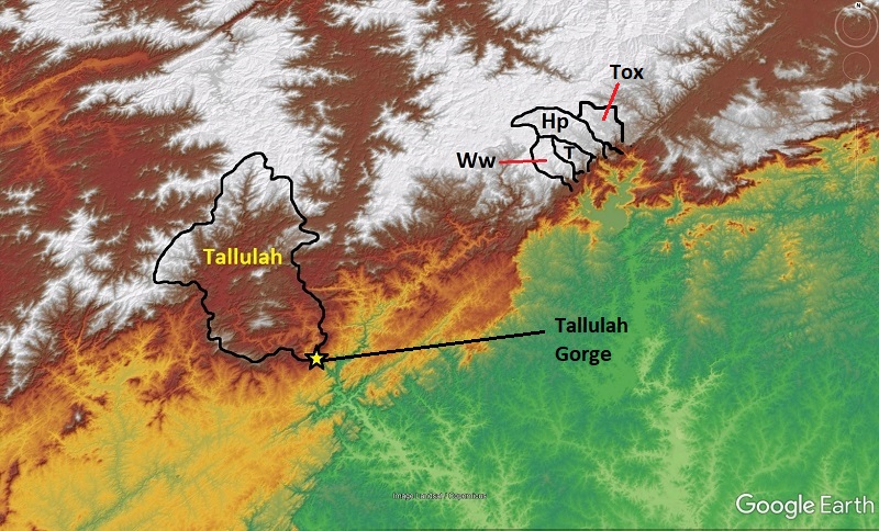
This impressive sequence of falls at the head of the gorge occurs where the Tallulah’s drainage area is ~190 square miles, or 500 square kilometers. When presented as a highly vertically exaggerated stream profile, shown below, the short but extremely steep stretch of river looks almost like a dam, and absolutely dwarfs every steep zone in the neighboring Chattooga River, a slightly larger river which the Tallulah meets just below its gorge. Not all of the Chattooga is shown here, but there isn’t anything Tallulah Gorge-like upstream of what is shown.
As far as I can tell, no other Appalachian river (at least in unglaciated areas) sustains a comparable gradient over 1 mile at a similar drainage area. Plenty of larger rivers have single waterfalls or sets of rapids (an example at the end of this post), but they do not approach the Tallulah’s sustained 1-mile gradient. Likewise, plenty of smaller named rivers descend more rugged topography and probably locally exceed the Tallulah’s gradient, but they are MUCH smaller rivers. The nearby Whitewater (Ww), Thompson (T), Horsepasture (Hp), and Toxaway (Tox) River basins are outlined below for comparison. Their combined drainage area would easily fit within the Tallulah basin.
The drainage area and gradient of Tallulah’s steep zone equate to impressive stream power that is not reflected in neighboring river systems. In many parts of the world, a large and atypically steep river like the Tallulah might be attributed to surface uplift due to active faults or landscape response to glacially-sculpted topography. Both of these factors are off the table in the Tallulah area. So, why is the Tallulah so big and steep? There are two reasons, and both become apparent with the aid of digital topography and geologic maps.
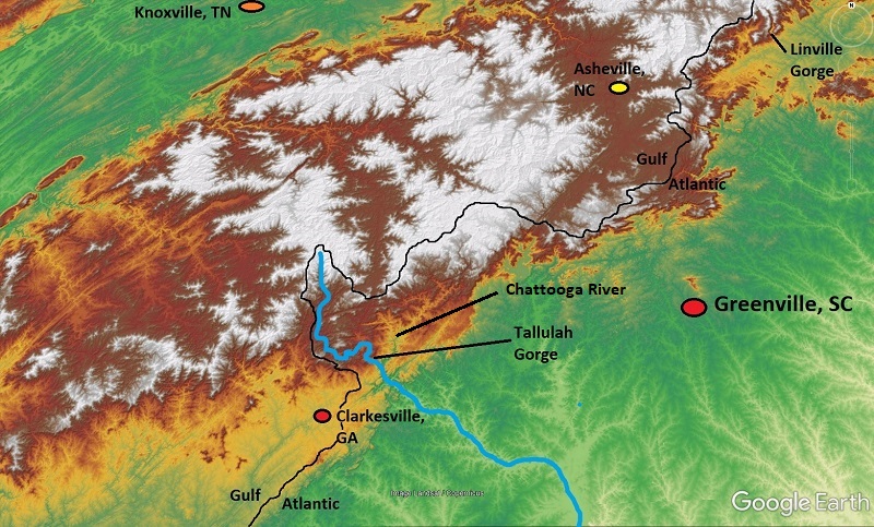
First and foremost, the Tallulah drainage basin has not always flowed to the Atlantic Ocean, a concept first noted by Johnson (1907). The Chattooga and Tallulah Rivers are the former headwaters of the Chattahoochee River system, which now drains the elevated plateau (yellow and brown) at lower left in the image below.
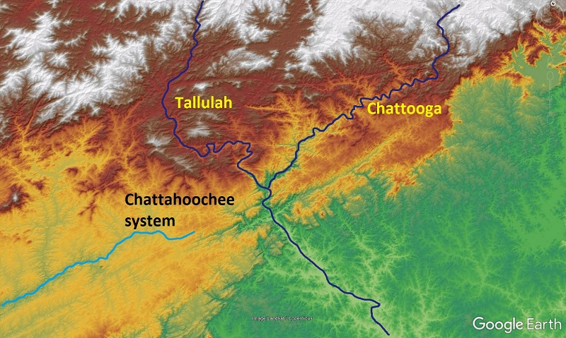
The old Chattachoochee headwaters loomed above the neighboring lower elevation stream networks of the Atlantic-draining Piedmont (green), creating a highly asymmetric drainage divide. Asymmetric divides are unstable over time, and headwaters of the Savannah system ate their way into the plateau edge, capturing the Chattooga and Tallulah and routing them off of the plateau into the lower elevation Savannah system. The GIF below animates the general idea of this process, which can otherwise be tough to visualize.
This stream capture event gave the Tallulah and Chattooga an additional ~660 ft (200 m) to descend, causing the rivers and their tributaries to begin carving deep gorges, which gradually ate their way upstream. The Chattooga (and any of its tributaries), however, don’t host any features like Tallulah’s steep stretch, which highlights Tallulah’s most significant aspect: its bedrock.
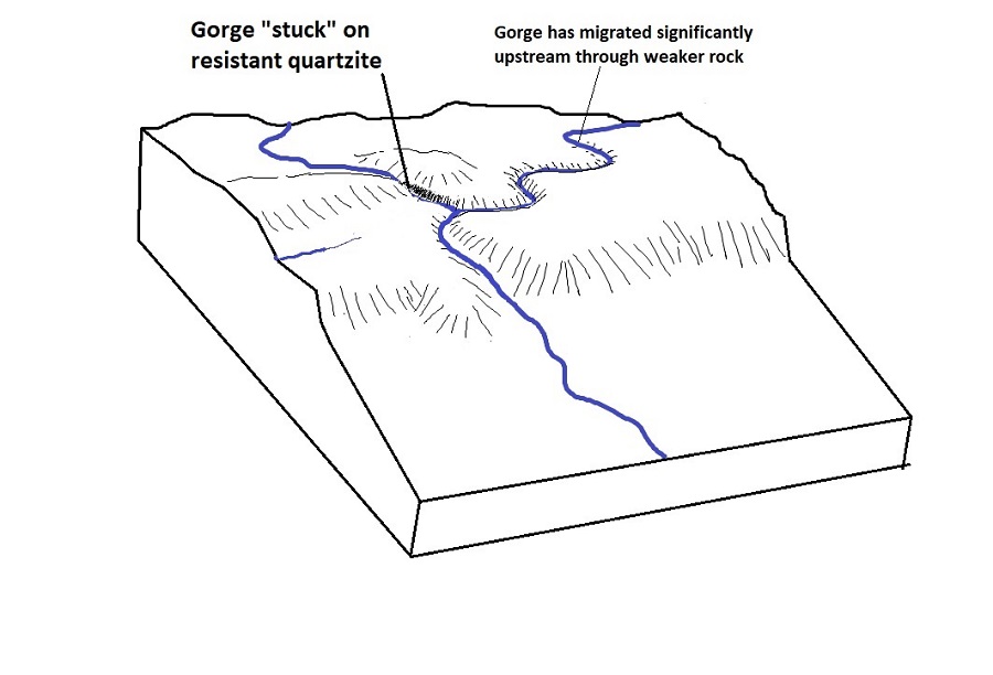
Tallulah Gorge is developed into quartzite, a metamorphic rock composed primarily of quartz (it’s not just a clever name). The quartzite, which is exposed within the Tallulah Falls Dome structure, is significantly harder/tougher/less erodible than surrounding rock types, and the Tallulah crosses plenty of it on its way to the Chattooga. In the GIF below drapes a great geologic map (Thigpen and Hatcher, 2009) over the Tallulah basin. Areas of quartzite exposure are yellow, and are widespread within the geologic dome. This map does a great job of showing the regionally atypical geology crossed by the Tallulah.
The quartzite bedrock is so resistant to stream erosion that the Tallulah has been unable to keep up with the Chattooga’s progressive downcutting in response to the stream capture. While the lower Chattooga has evolved towards a smoother transition into the rest of the Savannah system, the Tallulah has been comparatively unable to cut into its own distinct bedrock to match the Chattooga. As a result, much of the steepening related to the capture event is still “stuck” at the upper end of Tallulah Gorge, where the river is working hard to cut through the quartzite to allow the Tallulah to better match the Chattooga’s channel elevation.
This hard work takes the form of the large waterfalls, particularly the upper three falls, where the river is at its narrowest and its flow most concentrated. These falls represent the river concentrating its erosional energy as much as possible to try to catch up, erosionally speaking, to the Chattooga and the rest of the Savannah system.
The Tallulah’s work is made even more challenging by the downstream dip, or tilt, of the quartzite layers, which is particularly noticeable at Oceana Falls. I wore a GoPro while paddling in the gorge last November to film the short video linked here. Oceana is the first rapid shown (I run it twice), and downstream-dipping quartzite horizons are clearly visible to my left. Because of this orientation, the river is less able to access weaker horizons under the quartzite, which would cause undercutting and collapse of the hard layers. The block diagram below shows one interpretation (Hatcher, 1973) of structure beneath Tallulah Gorge. The geology shown here is very large-scale when compared to the size and depth of the gorge itself, but it does give an overall sense of structure. and the position of the gorge with respect to the only slightly exposed quartzite layers. Tallulah Gorge is presently located where the yellow layer starts to tilt down towards the right side of the diagram.
The quartzite (yellow, again) is not particularly thick. It is, however, in just the right place, and is dipping just the right way, to obstruct the Tallulah’s incision and force the river to become so atypically steep, despite its size and the relatively modest elevations of the surrounding landscape.
At the end of the day, the quartzite bedrock is really what sets the Tallulah apart and controls its unique steepness. The Tallulah’s valleys upstream of the gorge are notably higher than neighboring Chattahoochee valleys, suggesting a gorge and steep stretch of river has always been present where the Tallulah steps down from the quartzite into the surrounding landscape; the capture event has simply exaggerated this step. Without the quartzite, the Tallulah landscape would look much more like the neighboring Chattooga system, which drains schist and gneiss bedrock.
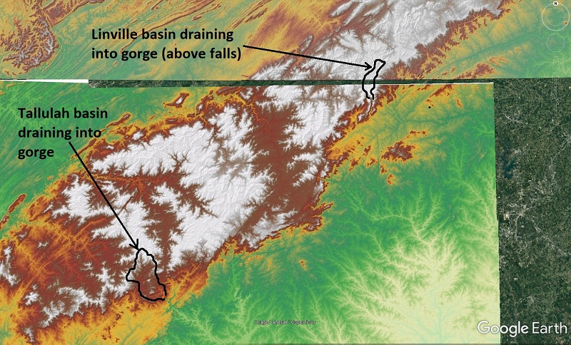
Quartzite always does interesting things in the Appalachian landscape, and the Tallulah is not the only river that interacts with this particularly tough rock type. Another noteworthy quartzite-crossing river is the Linville River, which is another stream capture victim. While the Linville descends farther than the Tallulah, it never matches the Tallulah’s one-mile maximum gradient. The Linville also drains a smaller area into the steepest portion of its gorge. Even so, the presence of quartzite within Linville Gorge absolutely impacts the length of the river’s steep stretch, presumably by slowing its downcutting and adjustment in a similar fashion to the Tallulah scenario.
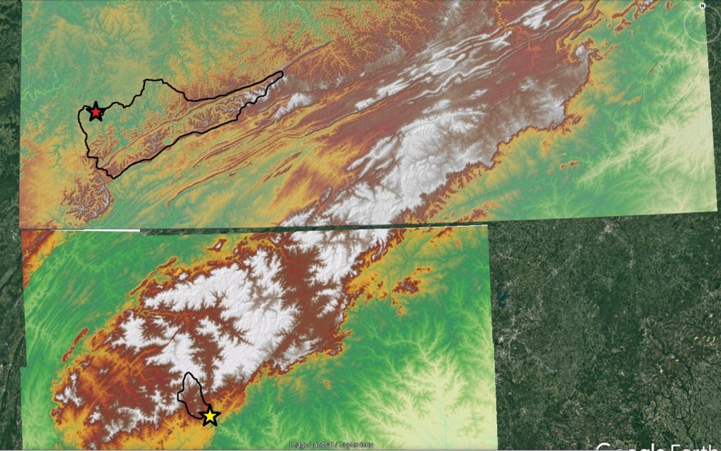
To repeat this post’s opening disclaimer, the Tallulah is noteworthy amongst rivers its size, but comparing it to significantly larger streams flowing over different bedrock is still an apples-and-oranges game to some degree. A river feature that has always impressed me is Cumberland Falls on the Cumberland River in Kentucky. This is a single, vertical waterfall is about 70 feet (22 m) high and occurs at around 2,000 square miles (5,200 square kilometers) drainage area. The image below shows the location of Cumberland Falls (red star) and the upstream drainage area, which dwarfs Tallulah (yellow star near the bottom).
Cumberland Falls is developed on sandstone overlying weaker shale, and is likely migrating upstream very quickly, geologically speaking. It is also the only feature of its type on the river, so the 1-mile scale steepness is nowhere near that of the much smaller Tallulah system. A direct comparison between Cumberland and Tallulah is complicated by completely different geologies and river system settings, but both are intriguing features that reflect geologic details of the host area.
The Tallulah River and its unique character are yet to be a significant presence in scientific literature, but I expect this to change in coming years. The gorge is dramatic in person, and its connection to geologic details makes it an equally impressive example of factors that control landscape appearance on Earth’s surface. I recently ran across a great Chattooga Conservancy website that gives some Tallulah history, including the great 1841 painting shown below. The painting appears to show the upper two falls and Hurricane, which is partly obscured at lower right. The faintly tan color used for the quartzite cliffs is a good representation of their actual appearance.
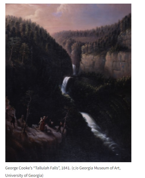
According to the Chattooga Conservancy site, an author named David Hillhouse wrote in 1819 that the falls of Tallulah Gorge were surpassed only by Niagara amongst rivers he had seen. I would say that there is geologic and topographic evidence to support his opinion.
-
“Squirrel tail” synclines in the Appalachian Valley and Ridge
by Philip S. Prince
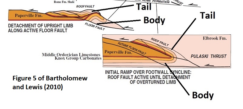
In the course of recent geologic mapping in the Appalachian Valley and Ridge, I came across a great 2010 paper by Jerry Bartholomew and Sharon Lewis describing extremely tight (and ultimately fault-transported) synclines in the footwall of a major Appalachian thrust system. I found myself in need of an analogy to describe the shape of these structures, and I settled on “squirrel tails” because Bartholomew and Lewis’ cross sections of the features reminded me of how a squirrel drapes its tail over its body and head. I am not sure if this is an effective comparison or not, but the overall approach seems to have served humans well when it comes to mentally organizing patterns of stars in the night sky. I provide supporting images below! (nice squirrel photo sourced here).

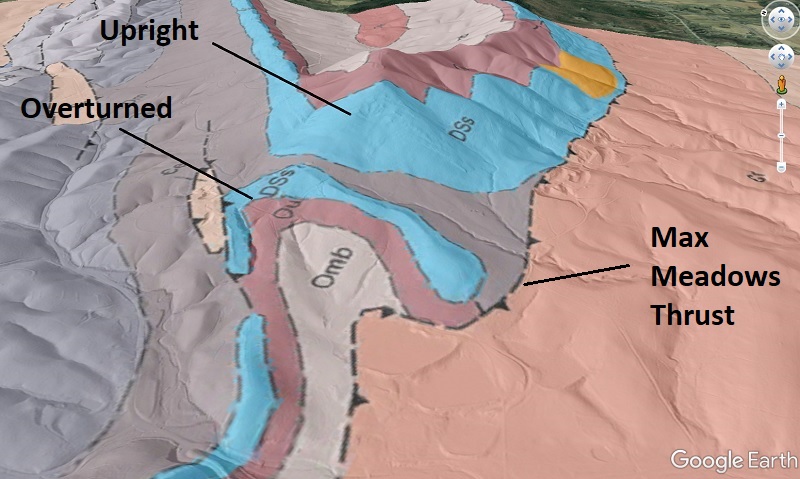
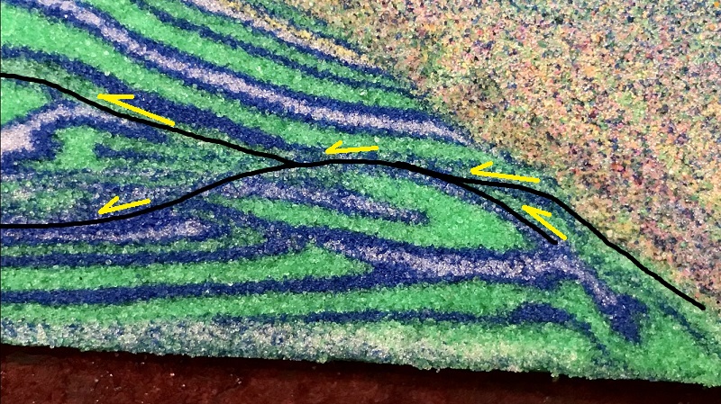
The squirrel tail type locality, which inspired the cross section above, is located between Radford and Christiansburg, Virginia, in the footwall of the Pulaski-Max Meadows Thrust fault system. This structural style came across my radar after I mapped a similar type of structure ~25 miles (40 km) to the southwest, near the town of Max Meadows itself. The geologic map overlay below shows the surface expression of the structure I mapped. Using the squirrel analogy, the overturned area is the tail, with the upright body still below it in the subsurface. The upright body portion is today exposed on Draper Mountain, which is labeled “Upright” below. This area stands out because the blue Siluro-Devonian sandstone unit is effectively folded back on top of itself, with apparently only a thin seam of Devonian shale (dusky blue separating the light blue zones) in between the upright and overturned limbs. The slightly synclinal overturned area is 2,000 ft (630 m) across at its widest, but would have been wider prior to erosion to present-day outcrop level.
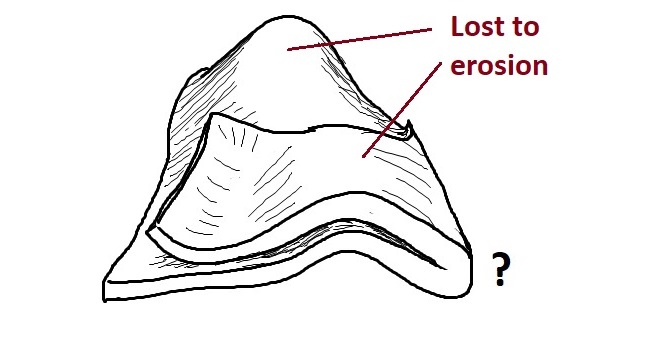
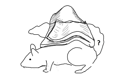
Surface outcrop patterns and lidar-derived hillshade maps suggest the structure of the blue Siluro-Devonian sandstone layer would look something like the sketch below, prior to erosion into its present outcrop pattern. The nature of the hinge area (the “?”–is it faulted?) is unknown. I “squirrel-ized” the sketch in the second image for comparison to Bartholomew and Lewis’ examples. Note that the sketch focuses on only one thin stratigraphic horizon; the pre-erosion structure, as well as the upright limb in the sub-surface, likely involve a bit more section. The Siluro-Devonain layer should also continue in the subsurface to the left/northwest; it is cut off here to illustrate only the folded area.
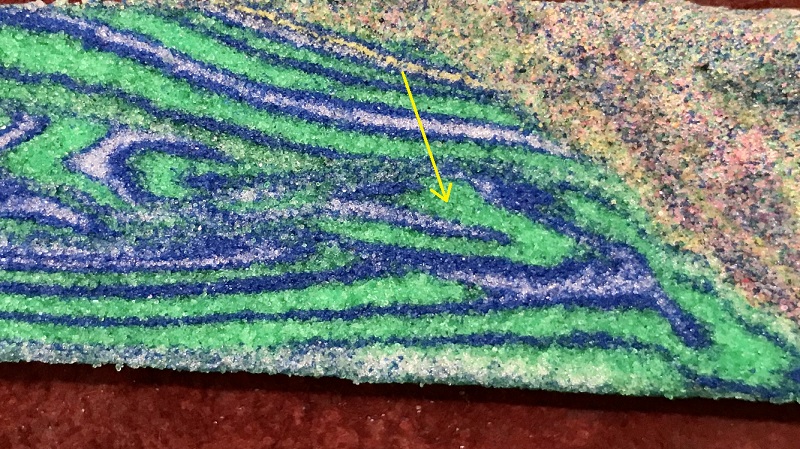
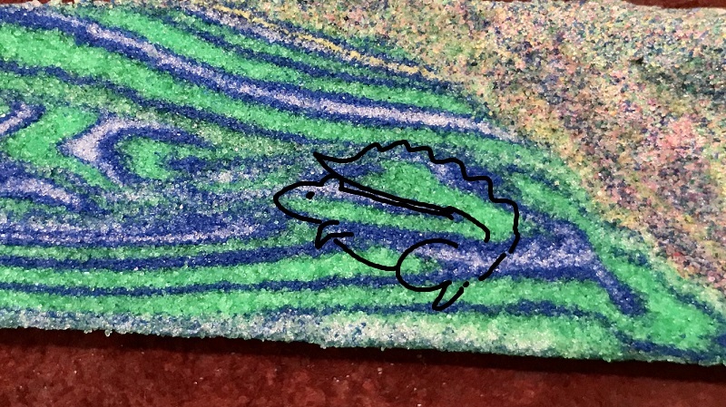
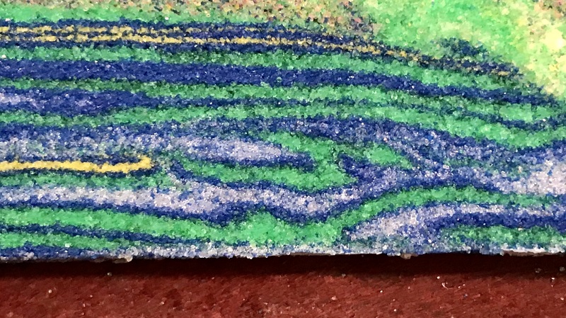
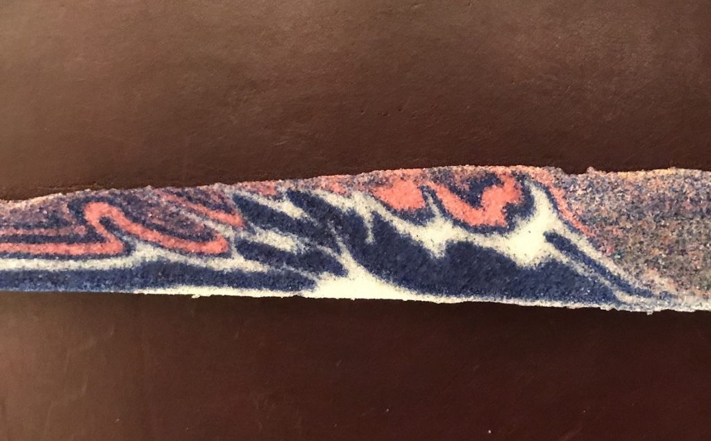
The mechanism through which such a lengthy overturned limb and tight overturned syncline develop is interesting to consider. I tried to create comparable structures in a sand model utilizing several overlapping weak detachment layers (white layers in the model images below). Surprisingly, I was able to produce tight footwall synclines that likely involved a single layer during their formation and initial fault transport. A good example is shown below, along with more squirrel-ization. Yes, this model is hopelessly green. Current supply chain struggles appear to affect colored sand, so only the shape of the structure is the focal point here!
I find this model complicated to look at compared to a nice set of colorful thrust imbricates, but I think it does contain a legitimate squirrel tail-type structure with upright and overturned limbs of comparable length. The limbs are separated by a very small amount of weak material. The structure occurs in the footwall of a major thrust system in the model, which is faintly arched by the underlying squirrel tail block.
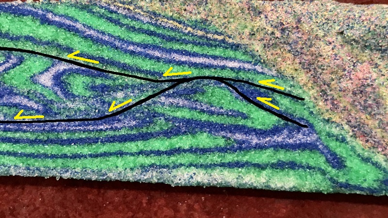
I can’t tell you how far the squirrel tail block was transported, as the strata from which it detached began to be thrust back over it as this portion of the model approached the rigid backstop. The right edge of the model also appears to have been damaged by extensional faults as the backstop was removed, but the squirrel tail was fortunately spared. The image below shows a larger view of the model and the context of the squirrel tail block. Its position near the backstop is comparable to that of the real-world squirrel tails, which occur in fairly close proximity to the outermost crystalline thrust sheets of the Appalachian Blue Ridge, which served as backstop to the Valley and Ridge sedimentary fold-thrust belt.
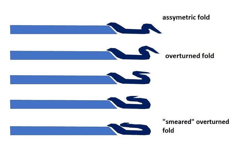
A primary goal of these models was to figure out what the overturning process actually looks like, as the long overturned limb cannot simply swing on a hinge like a door. Based on observations from a couple of other models, I think the overturned limb might develop through tightening and stretching of an early fold at the trailing edge of the future squirrel tail block. The sketches below attempt to illustrate this process. The overturned limb at Draper Mountain is massively damaged (veined and fractured) and only faintly stratigraphically recognizable, and I think the mechanism below would certainly produce extensive damage in the overturned limb.
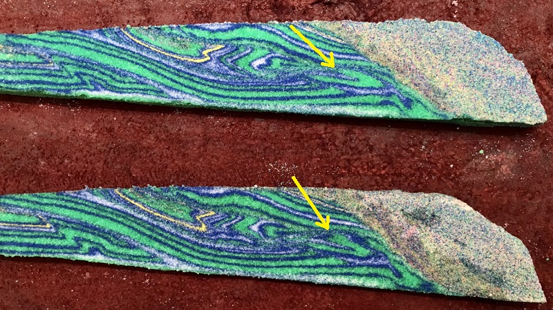
The model below may show the above mechanism in progress. Just below center, a developing squirrel tail is visible, lodged against the the yellow layer ramp (thrust transport was right to left). The overturned tail is not extensively developed yet, and it may show evidence of a tightening and smearing fold set as illustrated above.
I would love to watch one of these features form, but I can confidently say that I am very unlikely to produce one of these features in a model with glass sidewalls. These models also require a large amount of shortening to fully develop, and they rapidly become prohibitively large and heavy due to the volume of sand and microbeads necessary. I haven’t completely abandoned this setup, however, and I plan to try a few more to see what other types of major thrust footwall structures can be developed.
-
Lidar unboxing day: A few southwest Virginia treats within ~1 hour of Blacksburg and Virginia Tech
by Philip S. Prince
I always look forward to my first look at high-resolution lidar imagery from a familiar area. Last week, I took time to check out some some new-to-me imagery from areas surrounding Blacksburg, Virginia, where I spent about 10 years studying and then teaching at Virginia Tech. I found the following features particularly interesting, as I have regularly viewed or even walked across all of them without appreciating their presence!
- Huge, historically (<100 years) or currently active debris slide, New River above McCoy Falls, Pulaski County
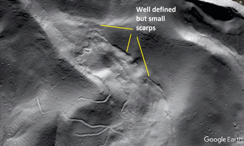
This slide, which resembles a glacier creeping down towards the river, has developed in the debris pile produced by a large rockslide on Walker Mountain. The rockslide laid bare white cliffs of Tuscarora Sandstone that I have always heard called “White Face.” The rockslide is ancient (Pleistocene?), but activity in the resulting debris pile is much younger. The GIF below shows the slide and its topographic context. White Face is visible at the very top center in the aerial photo image. The curving path of the slide can be appreciated from this perspective. I have looked across the river at this area hundreds of times, so this 1-meter hillshade view is very satisfying!
To me, the most striking feature of the slide is the crispness of its lateral scarps and headscarp. They don’t appear to be very large, but remain very crisp and well defined, suggesting recent or ongoing activity.
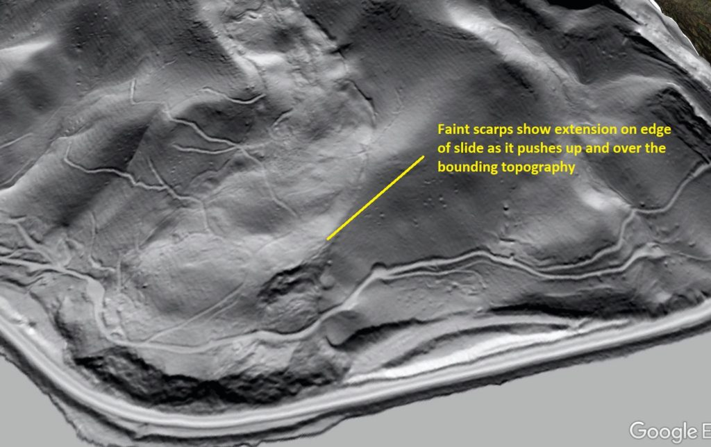
The edge of the slide can be seen cracking along the left-lateral scarp as material pushes up and out of the topographic low that holds the debris deposit.
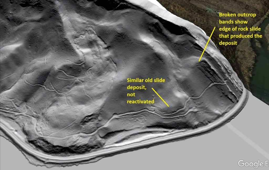
I can’t personally speak to the movement history of the slide, but I suspect that removal of a portion of its toe to construct the railroad running along the river may have led to reactivation. A smaller slide to the north (right side of the image) was not altered by railroad construction, and looks very old and stable compared to its large neighbor.
2. Rock blockslide along Big Reed Island Creek, Pulaski County
This slide has experienced little displacement, but lidar reveals an impressive graben that is forming as a large mass of Hampton Shale (really a slate or phyllite here) bulges outward from the riverbank as it is undercut by Big Reed Island Creek. The slide and graben are at the center of the image below.
The graben and slide are, unsurprisingly, invisible without a lidar-based image.
The graben is quite large compared to the overall scale of the slide. I think this indicates that the basal sliding surface slopes less steeply than the land surface, meaning the slide mass is thick and deep, particularly at its upslope end. The block diagram below attempts to illustrate this idea.
This slide is included on the Hiwassee quadrangle geologic map (linked here), and structural data indicate the failure is occurring along the crest of an anticline that plunges northeast. The basal sliding surface could therefore be a bedding plane/foliation plane failure whose low dip is an expression of where it sits within the fold structure,. The orange form lines in the diagram generally indicate layering orientation as it might appear on this cross section cut, which is at an angle to the fold axis.
I actually went to the foot of this slide with Virginia DGMR geologist Matt Heller during a canoe transect of the map area in June 2019. The poor photo below shows what the downslope end of the slide looks like, right above Big Reed Island Creek. This huge outcrop sheds plenty of rock, and does not feel like a place you would want to stand around for too long.
3. Buck Hollow Ridge rock slope deformation, Macks Mountain, Pulaski County
This slope movement is not far from the Big Reed Island Creek feature, and occurs in Erwin Formation quartzite just up-section from the Hampton Shale. Sub-surface failure within the Hampton Shale may have actually caused the movement, but I don’t know for sure.
This failure indicates the precarious stability of some rock slopes (particularly dip slopes) in this part of Virginia, even if they host resistant rock types like quartzite. I have hiked along the toe of this feature before, and never knew it was there. The logging road grade along the summit cuts right through numerous scarps. I think this feature is particularly interesting because the headscarps are found on the back side of the ridge crest, meaning the summit of Buck Hollow Ridge has lowered slightly due to the failure.
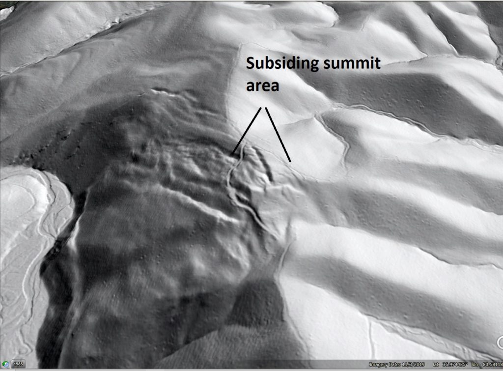
The slide has developed on a dip slope, with slate/phyllite beds being the likely seat of the basal failure. Dipping quartzite beds nearer the surface are visible in the lidar imagery, as are subtle flatirons within the landscape around the slide. Progressive undercutting of the toe by Big Laurel Creek may have kept this sliding intermittently active for a lengthy period. It makes me wonder what a large-scale, man-made cut along the toe might do…

4. Folded Chilhowee quartzite beds on Poor Mountain, Roanoke County
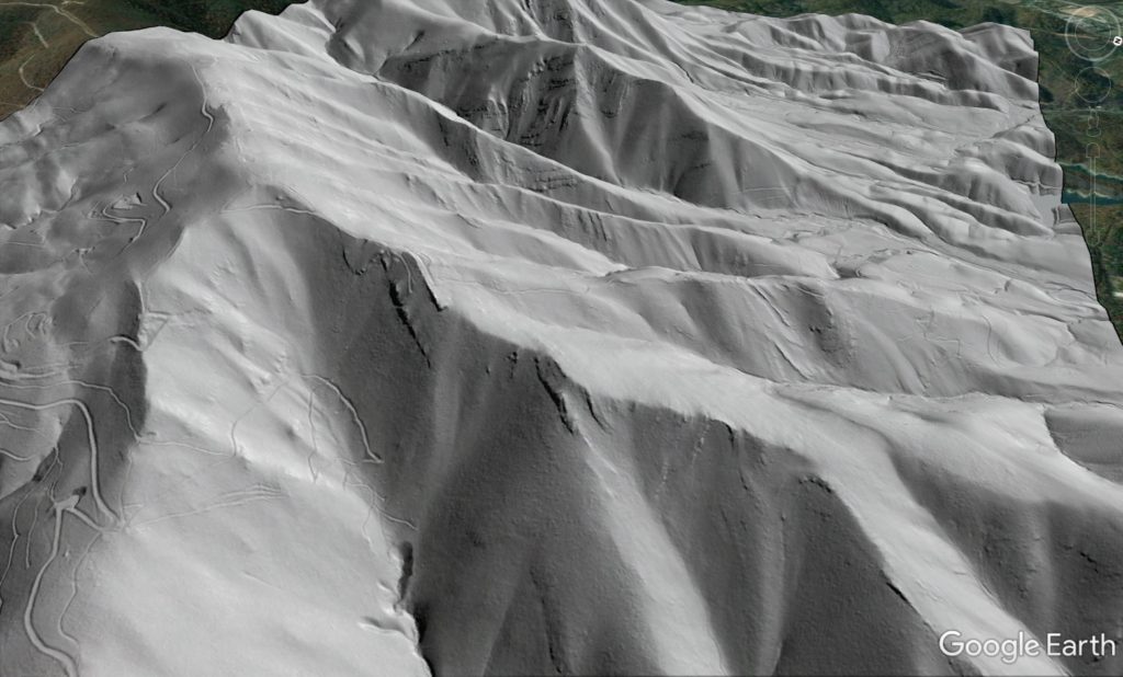
Poor Mountain is topographically impressive. It absolutely looms above Interstate 81 south of Salem. Despite its size and steepness, its slopes are mostly forested and minimal outcrop is visible. Lidar hillshade imagery shows nice folds in the basal Cambrian/latest PreCambrian Chilhowee quartzite that supports Poor Mountain’s steepness and elevation.
The obvious folds extend about 2,000 ft (600 m) over the land surface in the image above. Their amplitude is exaggerated because they are viewed on a slope and not in a vertical cut, but folding is definitely present. The yellow lines in the image below approximate contours on the land surface, and beds can be seen to cut steeply across contour before paralleling it, and then cutting across it again.
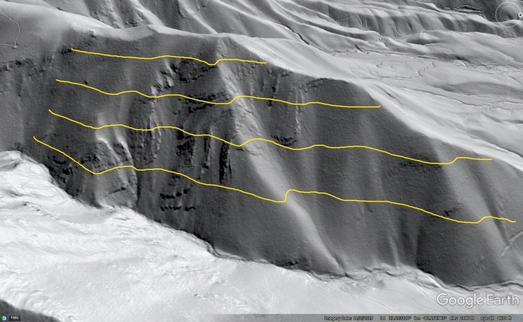
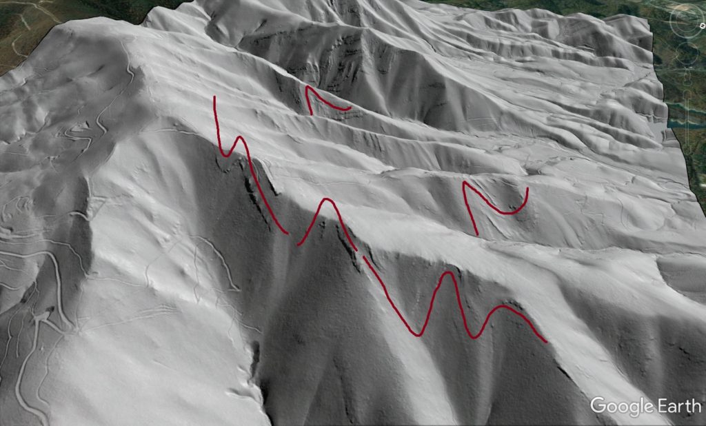
Folding is extensive in the Chilhowee is extensive across the northwest face of the mountain. The lower image below uses lines to call out some of the structures in the foreground.
5. Rock Castle Gorge rockslide, Patrick County
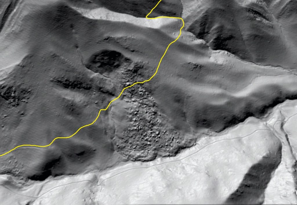
Rock Castle Gorge is actually named for clusters of terminated quartz crystals found in the area, but its Blue Ridge Escarpment location makes it a very rough and rocky place at the larger scale. A main loop hiking trail through the gorge passes through the upper portion of the rockslide shown below, which is conspicuously bouldery and rocky to an observer on the ground.

The still image below shows what I believe to be the route of the hiking trail. I have walked the trail several times, though not for a number of years.
The texture of the slide mass shows the presence of different materials, which are likely schists and amphibolites. The chunky, bouldery material appears to overlie less bouldery material, and is also partly buried by less bouldery material derived from upslope. The bouldery material is clearly derived from the resistant horizon cut by the slide. I have tried to delineate these material-specific zones below.
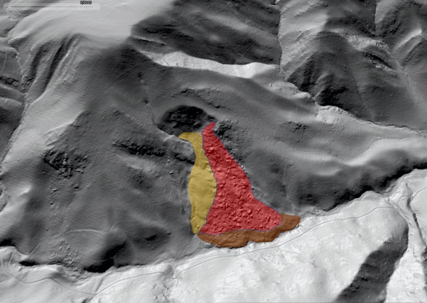
A visit to this feature would quickly indicate how the stacking order of material in the slide mass reflects position of the in-place materials on the slope. Whether this slide is the result of a single failure or successive failures is unclear. It is also somewhat unique in the area. Despite its steepness and the frequent occurrence of dip slopes, the Blue Ridge Escarpment and its intensely folded metamorphic outcrops seem to host far fewer landslides than the folded/faulted sedimentary Valley and Ridge to the west.
-
What does that landslide actually look like, part 2: an active landslide
by Philip S. Prince
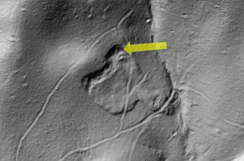
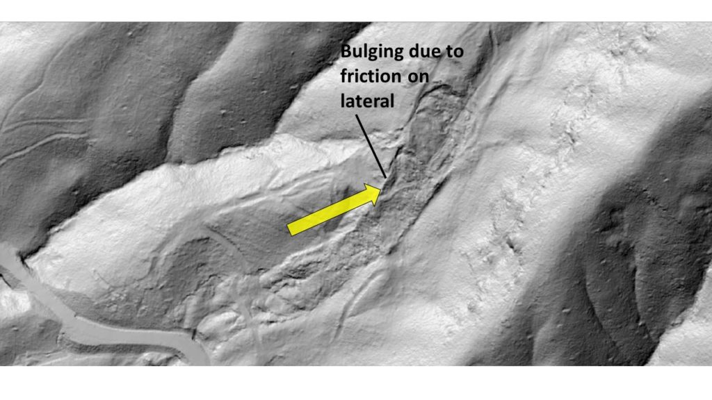
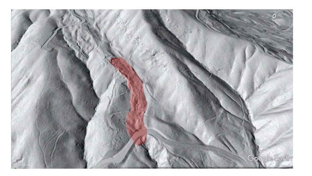
As indicated in the previous post, lidar-derived imagery still needs ground-truthing to maximize its usefulness as a means of characterizing landslides and other slope failures. Last June, Ken Gillon and I visited the Rutherford County, North Carolina, landslide described below as part of our work with Appalachian Landslide Consultants, PLLC (ALC) on behalf of the North Carolina Geological Survey. This slide caught my eye in lidar hillshade imagery because it appeared to share characteristics with an active slide we had visited a few days before. Compared to the slide in the last post, this slide is very subtle in its lidar appearance, due in part to its location in a topographic hollow. For its first appearance in this post, I have highlighted it with a transparent red overlay.
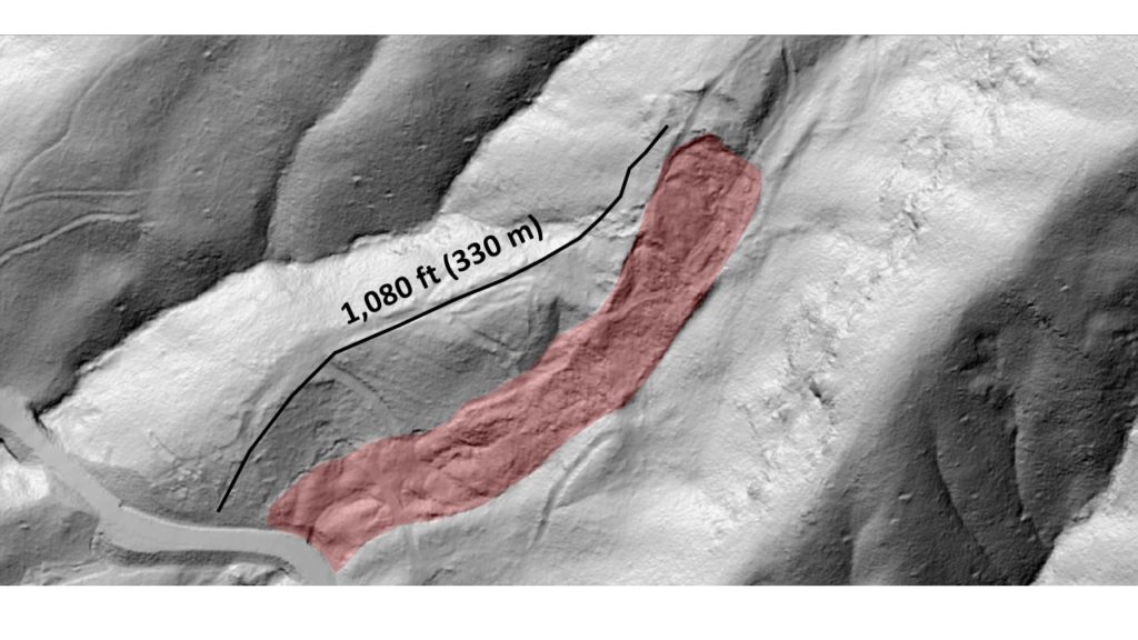
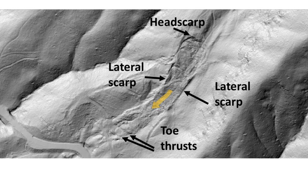
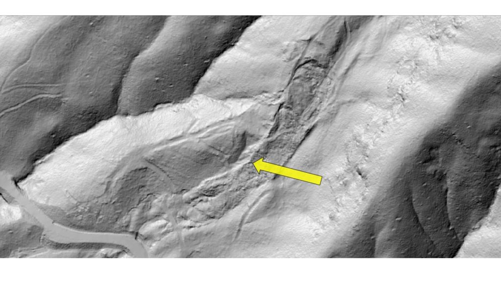
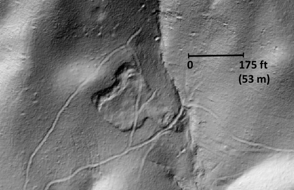
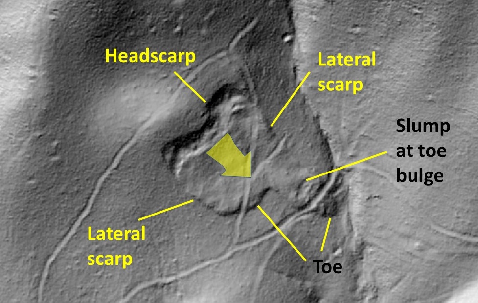
Without the red overlay, the slide may be somewhat difficult to pick out for those who do not evaluate lidar-derived imagery on a daily basis. It is shown without the overlay below, but notable kinematic features are labeled. The faint orange arrow indicates its direction of downslope movement.
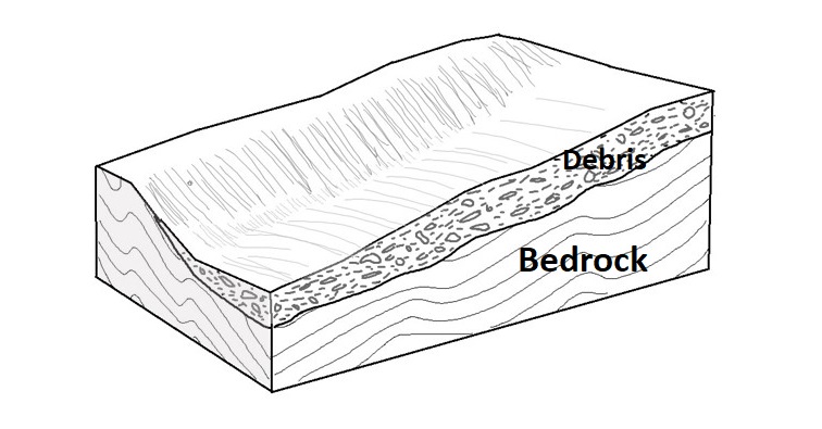
Like the slide in the previous post, this is a debris slide in which rock fragments and boulders derived from nearby steep slopes and cliffs are almost certainly sliding atop underlying bedrock. If the debris deposit is particularly thick, the sliding surface may be entirely within the debris. In either case, the debris is dominated by platy fragments of amphibolite rock. The shape of the amphibolite fragments allows them to slide past each other easily. The position of the slide in a topographic hollow makes it very wet, which also favors sliding. The conceptual drawings below illustrate the general debris slide idea, with the red lines in the lower image highlighting sliding surfaces. Note that they are highly vertically exaggerated compared to the real slide.
While it is unimpressive in lidar hillshade imagery, this slide was fascinating to visit in the field. It is presently active, although it is moving very slowly and probably episodically. It displays a number of features associated with slow, active landslides that are always interesting to observe in the field. The photos below highlight some of these features. Each is preceded by a lidar hillshade image showing the photo location, with the point of each yellow arrow resting on the photographer’s position. The general pointing direction of each arrow indicates the direction in which the photographer was looking. The images also provide a nice glimpse of what fieldwork looks like in Rutherford County, North Carolina, in June!
After entering the woods from the road downslope of the slide, the first indicator of slide activity is trees being pushed over by the toe of the slide. Ken provides a scale reference in the photo below.
Most of the trees being pushed over are young because this part of the slide was logged within the last ~25 years. This may have contributed to the slide’s present activity, but this is impossible to confirm. Each of the toe thrusts visible in the lidar imagery displays tree push, suggesting all the toe thrusts are actively (but slowly) moving.
The toe thrust structures are associated with minor uplift and bulging of the land surface. As the toe bulges grow and curve, their crests stretch and crack, resulting in open cracks and fissures. In the image below, Ken is seated next to one. Forward-rotated trees are visible next to him; these have not been physically knocked over. Platy fragments of amphibolite are also visible on the margins of the fissure. The photo below was taken very close to the one above.
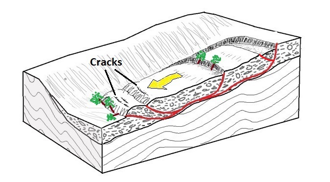
This fresh fissure development or cracking is interesting evidence of slide activity, and the width of the toe bulges indicates that the slide mass is certainly several feet (more than 2 meters, for sure) thick here. The conceptual drawing below shows the location of the fissures or cracks atop the toe bulges. I have also included some trees knocked down by the slide toe, directly below the word “cracks.”
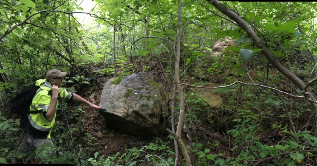
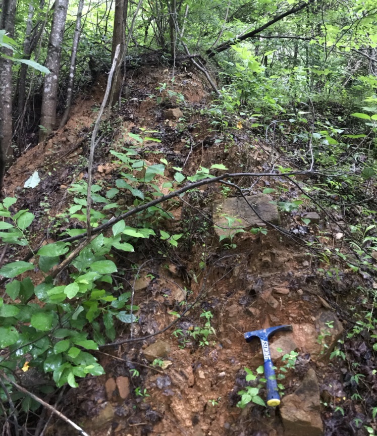
Bulging at toe thrusts also produces locally steep slopes, causing large rock fragments and boulders to dislodge from the steepened area. The boulder in the image below was one of several that had recently dislodged, exposing stained surfaces that were once seated in the soil.
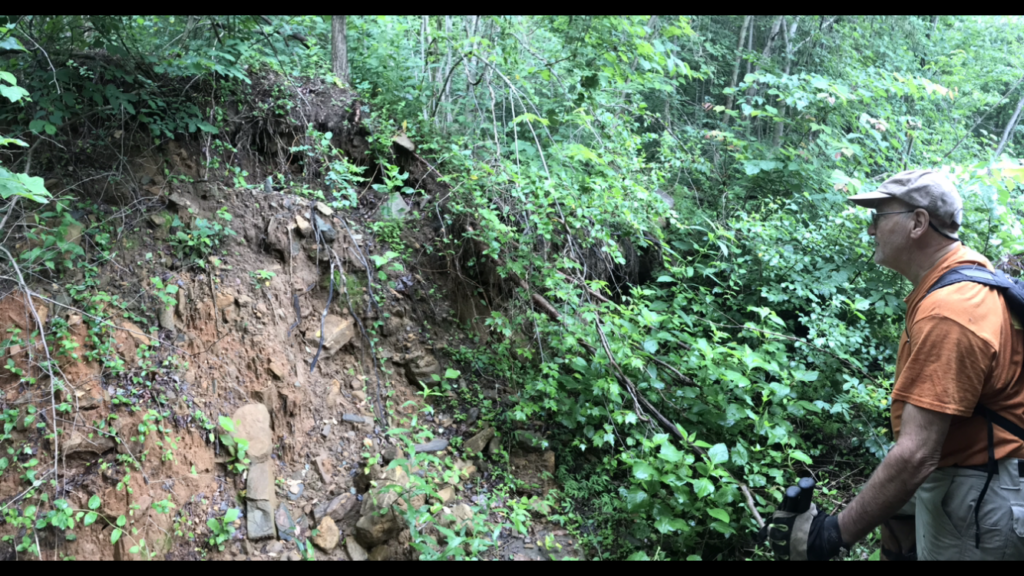
The slide has numerous internal scarps that may result from its movement over an uneven bedrock surface. They may also represent separation and independent movement of single blocks with the overall slide mass. The scarps provided a good look at the debris composition of the slide mass. The next photo shows an internal extensional scarp, somewhat like the one near the middle of the slide mass in the drawing above.
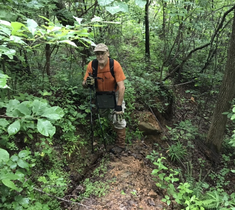
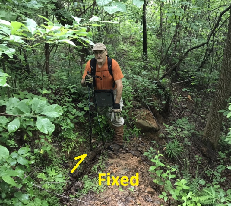
The lateral scarps of the slide displayed local bulging due to their friction against the fixed surrounding ground. The photo below shows the downslope end of one uplifted area.
The crest of the uplifted area (near the end of the black pointer line in the lidar image above) displayed a well developed and very crisp surface crack. It is visible at Ken’s feet in the photos below.

At the upslope end of the lateral bulge, an impressive lateral scarp was visible near its transition into an internal extensional scarp/headscarp. This scarp was very fresh and crisp, and I thought it appeared locally grooved and striated due to the motion of the slide mass that exposed it. These features are not readily discernible in the next photo.

At the uppermost active headscarp of the slide, a broad depression has developed. The depression is likely the surface of a graben, or downthrown block of material bounded on each side by shear surfaces. Trees with root structures compromised by development of the depression were falling in all directions in this area.
The conceptual drawing below shows the position of the graben within the overall slide mass. The scale of the graben on the real slide suggests it might be over 10 feet (over 3 meters) thick in this area, but no field evidence was available to support this.
Even though this slide is not particularly impressive in lidar imagery, it has the potential to be impactful should the immediate area experience any type of development, either infrastructural or residential. The area affected by the slide is, of course, unstable and unsuitable for building. The slide is quite large, and it is unlikely that any sort of engineering work would be able to stabilize it, particularly due to its overall wetness. Its slow motion, however, could make it deceptive to developers who might not pick up on the landscape features described in this post. It is certainly plausible that the area could be cleared and locally graded and construction of a home at least begun (if not completed) before the slow slide movement began to produce very noticeable, irreversible damage. The land surface above the toe of the slide in all of the lidar images is, by contrast, stable, as it is underlain by weathered bedrock with some outcrop. It is perfectly suitable for construction. The area to the right of the slide, which is below cliffs and steep outcrop, is also unsuitable due to its potential to experience future slide movement or rockfall.
This slide is not unlike a wet “glacier” of rock debris that is slowly creeping its way down the ravine. The perspective of the image below shows the position of the slide with respect to the surrounding topography, as well as its slightly curving path.
Ken and I encountered a few of these active amphibolite debris “glaciers” last summer. It was not possible to definitively determine the reason for their activity, but all were in topographic ravines and hollows, and were thus very wet. All were dominated by platy rock debris, the fragments of which could easily slide past one another. All had experienced logging in recent decades as well. Presumably, the combination of these factors contributed to the slow but ongoing movement of these slides. As far as the slide in this post is concerned, road construction may also have contributed to its reactivation. In the lidar image above, an area below (downslope) of the obvious road grade appears to also be part of the slide mass which is now disconnected by the roadcut. Construction of the roadcut may have destabilized the lower part of the slide mass, causing reactivation to spread upslope. Ultimately, we will never know the specific cause of this or many of the slides in the area, but we definitely know that they are worth avoiding for construction and engineering purposes!
Like so many Appalachian landslides, this one is completely hidden by vegetation for much of the year. It is located near the center of the GIF below, which is comparable to the extent of the lidar image above.
(DEM imagery captured from QL1 lidar data acquired by NC Dept. of Public Safety, raw point clouds assembled and processed by Corey Scheip of the NC Geological Survey Landslide Hazards Program)
-
What does that landslide actually look like?
by Philip S. Prince
Lidar-derived imagery is a game-changer in the study of landslides and other slope movements, and it frequently produces dramatic visuals like the Rutherford County, North Carolina, debris slide shown below. The slide has developed in talus dominated by sillimanite schist, which is likely sliding atop underlying gneissic bedrock.
Over the past year of focused landslide mapping here in southern Appalachia, I have noted that slides that are this crisply defined in lidar hillshade are often found to be active upon field inspection, with soil-exposing scarps, ground ruptures and fissures, and trees back-rotating or being pushed over. The (very) humid temperate climate of the region is not well suited to preserving the fine details of many landslides, particularly when they do not involve intact bedrock masses. Numerous kinematic features are beautifully defined on the slide, with detail on the slide’s toe and laterals being particularly impressive and comparable with confirmed active slides in the area. The slide is equally dramatic using slope-shade imagery, which can offset bias effects related to lighting angle in hillshade imagery.
I recently visited this slide as part of my work with Appalachian Landslide Consultants (ALC), PLLC, and was surprised by its actual field expression. The following photographs show what the slide looks like in the field. The accompanying hillshade images show where each photograph was taken, with the points of the yellow arrows resting on the photographer’s position (this is to avoid covering the details of the slide with the arrow). Each arrow points in the direction the photographer was looking.
Surprisingly, no bare soil was exposed on the scarps of the slide. The headscarp is shown below. Up and right from the center of the photograph below, ALC geologist Aras Mann is seated on the scarp surface. Trees show minimal deformation here.
Many of the trees growing on the headscarp are very young, suggesting its re-vegetation may be quite recent. Even so, it is presently entirely vegetated with an O-horizon present everywhere.
The toe of the slide is impressively defined in lidar hillshade, but it is much more subtle from the ground surface. In the photograph below, Aras contemplates the surprising field appearance of the toe. The dashed yellow lines highlight the faint step on the land surface. The few leaning trees behind Aras are located just beyond the tip of the yellow arrow, where a portion of the toe appears to have slumped slightly due to oversteepening.
The toe bulge is certainly large enough to be noticed, particularly if one already knows that it is there. The bulge is about 6 feet (1.85 m) tall where it is crossed by the logging road. Note the two dead (or dying) trees at the right of the image…could they be evidence of creep within recent years?
Notably, the logging road does not appear to have been deformed by any noticeable slide movement.
Looking back upslope toward the toe from a logging road further downslope, only a faint step in the landscape is visible. The photograph below was taken from the logging road (point of the arrow). Again, the yellow dashed lines highlight the step.
The outermost portion of the toe (lower right of the slide in the images) has slumped due to oversteepening. The resulting headscarp is visible in the landscape in the photograph below (dashed yellow lines again). Some fallen trees were present here, but I did not consider them obviously attributable to slide movement.
The transition from toe to left-lateral scarp was also surprisingly subtle. Again, the toe bulge was large enough to be noticeable, but the crisp lateral visible in lidar hillshade was mostly obstructed by tree growth.
Interestingly, a similar pattern of dramatic lidar appearance and subtle field expression was observed elsewhere in the area. About 1,000 feet (300 m) northeast, another eye-catching (in lidar, at least) debris slide was found to be similarly vegetated. The slide described above is located down and left of center in the image below; its neighbor is pointed out just right of center.
This is another debris slide with crisp scarps and interesting patterns related to extension in the interior of the slide, near the center of the image.
Field investigation revealed another completely forested slide with no clear evidence of recent or ongoing movement. Older trees on the steepest portions of scarps showed some curvature, but, again, this slide looked nothing like what we expected. The slide does maintain several closed sags and depressions, although they too are completely forested. In the photograph below, Aras is standing in one such depression just below the western headscarp of the slide.
The slope which hosts these two slides is home to several other debris slides, all developed in the schist talus. The schist is well foliated, with fragments maintaining surprisingly planar and smooth foliation surfaces which easily slide past each other and along the underlying bedrock. Other slides are pointed out in the GIF below.
Many are equally well defined in lidar, and are similarly vegetated and unremarkable in the field. We have no constraints on the age of the slides, but they may reflect logging history in the area. The majority of these slopes were heavily and continuously logged during the past ~150 years, with logging in this area clearly occurring within the past 50 years. The slides may have developed after clear-cuts, with the rapid return of vegetation common in the region quickly making the area look less disturbed than it really is.
(DEM imagery captured from QL1 lidar data acquired by NC Dept. of Public Safety, raw point clouds assembled and processed by Corey Scheip of the NC Geological Survey Landslide Hazards Program)
-
The Ray Sponaugle well: A 13,000 ft lesson in Appalachian Valley and Ridge structure
by Philip S. Prince
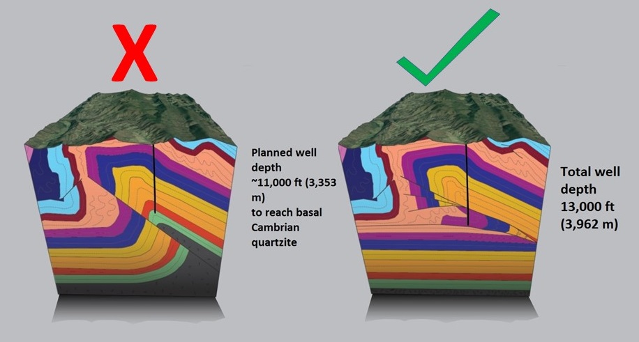
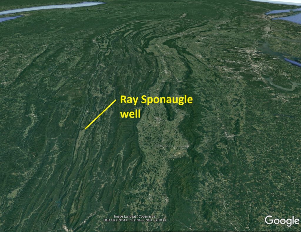
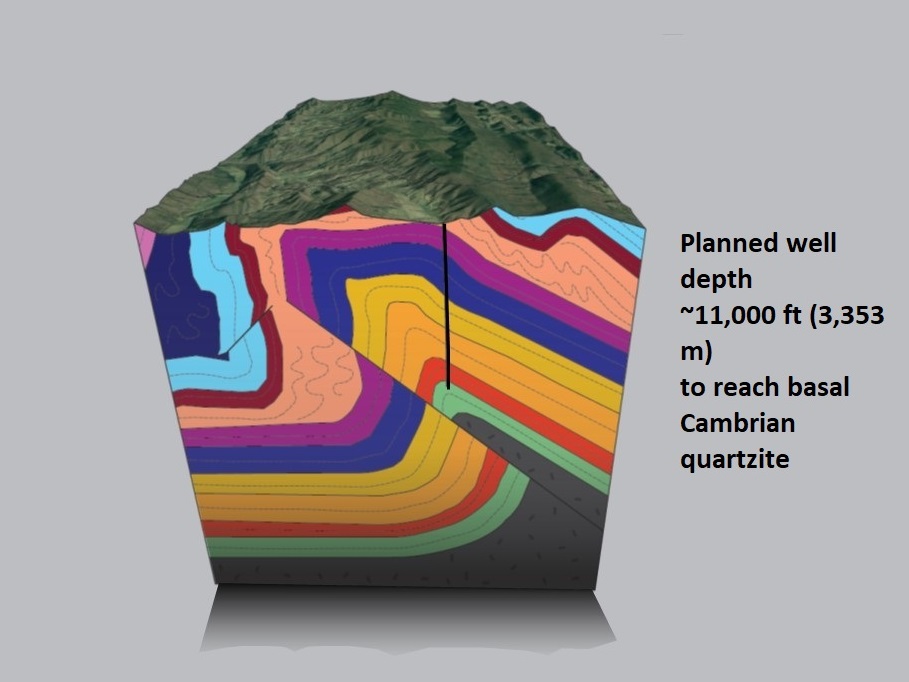
The 1964 Ray Sponaugle #1 well of Pendleton County, West Virginia, did not produce any hydrocarbons, but it did provide essential information about the structural details of a major Appalachian Valley and Ridge anticline and sedimentary fold-thrust belts in general. The well was intended to target lowermost Ordovician- and upper Cambrian-aged carbonate layers beneath the Wills Mountain Anticline, a major structure at the leading edge of the zone of significant folding and faulting in the Valley and Ridge. The well was expected to terminate in Cambrian quartzites at slightly less than 11,000 ft (3,353 m) below the surface.
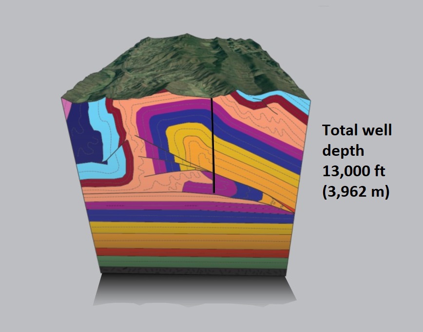
To the surprise of the drillers and geologists involved with the project, the well bore never got anywhere close to the Cambrian quartzite. At 10,000 ft (3,010 m) below the surface, the well passed through a thrust fault and entered a tight, nearly recumbent syncline cored by the same Ordovician shale unit into which drilling began. Ultimately, after 13,000 ft (3,962 m) of drilling, the well was terminated in a horizon of rock equivalent to layers the well first passed through only 1,300 ft (396 m) below the land surface. The block diagram below shows this basic structure; the heavy black vertical line is the approximate well bore. The basal Cambrian quartzite layer (green) was probably 8,000 ft (2,438 m) or more below where drilling stopped. Pre-drilling understanding of Valley and Ridge structural style was obviously a bit off target…
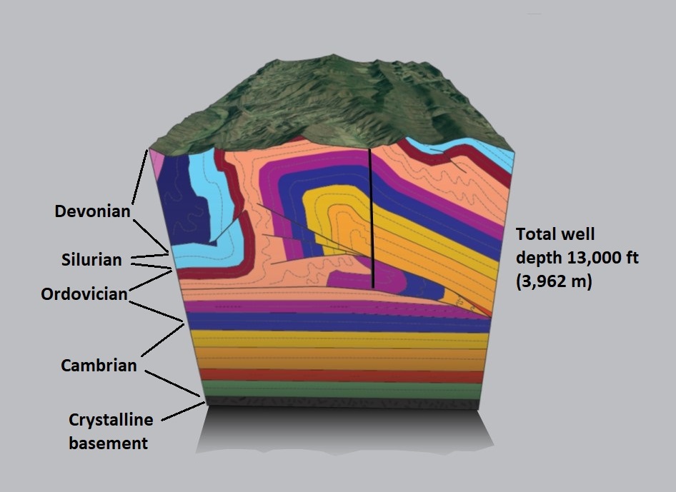
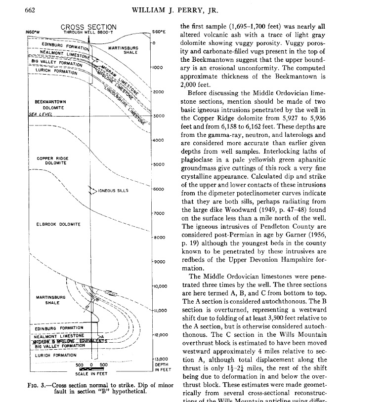
I drafted this block diagram from Google Earth surface imagery, a partial cross section from William A. Perry, Jr.’s 1964 AAPG Bulletin article describing the well, and Kulander and Dean (1986). The purple layer is the Middle Ordovician limestone interval through which the well bore passed near the surface and ultimately terminated in at 13,000 ft total depth. Perry’s description of the well, accessible here, is a fascinating read, and one can genuinely sense his surprise at the outcome, largely due to drilling so far to reach the same rock layers the well passed through much closer to the surface. Perry’s small cross section from the paper is shown below.
While the geometry shown in this cross section and in the block diagram would be considered a very reasonable Valley and Ridge (or any “thin-skinned” sedimentary fold-thrust belt) structural style today, conceptual models of Appalachian Valley and Ridge geometry were somewhat different in 1964. Drilling was expected to encounter the Cambrian quartzite (green in the block diagrams) at just under 11,000 ft (3,353 m) deep because faulting beneath anticlines was believed to involve crystalline basement rock (gray in the diagrams) and cut across sedimentary layers at constant angles, regardless of the mechanical properties of the layers. I tried to re-work the block diagram to illustrate this prediction, basing the geometry on some papers from the time.
Compared to the actual structure revealed by drilling, the source of Perry and others’ surprise is evident:
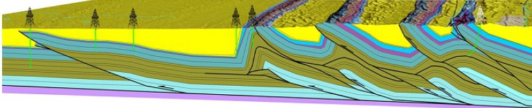
The Sponaugle well showed that faulting could localize within (and propagate parallel to) weak shale layers, allowing portions of the sedimentary section to detach, fold and fault above and independent of the basement rock. Faulting did not cut through the entire section at a fairly constant angle all the way down to crystalline basement (see the Cooper section at the end of the post). The structural style revealed by the Sponaugle well also provided a way to account for rock volume inside of anticlines by stacking and repeating large, shale-bounded portions of the stratigraphy without using basement rock and the full sedimentary section moving together. Perry rightfully deemed it necessary to reconsider Valley and Ridge structure at all levels. This was one of many steps towards the adoption of the “thin-skinned” model for the Valley and Ridge, in which major thrust faults sole into a Cambrian shale decollement (detachment) and step up into younger shales, independent from deeper Cambrian units and basement rock. Analogous thin-skin style geometries can be replicated in physical models containing weak layers to serve as decollements.
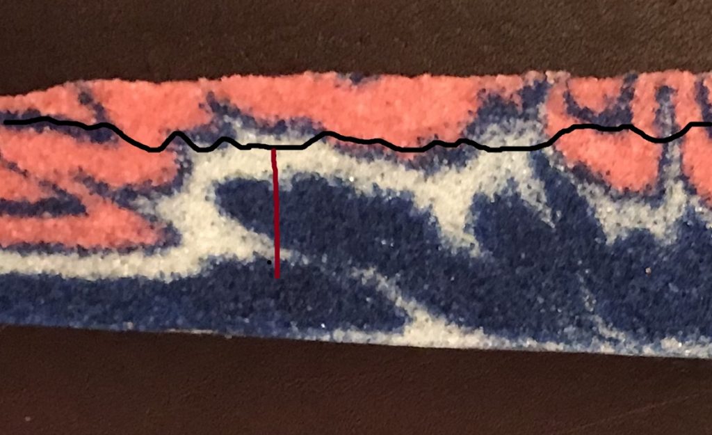
In the model above, the white layer at the base of the section is the master decollement, representing the detachment between the layer pack and the fixed base on which the model was produced. The mid-section white layer will also develop very low angle, nearly flat fault segments that connect steeper faults cutting the blue and pink layers. Working together, the two weak white layers allow the blue layer to be stacked on top of itself. A well drilled in the center of the frontal anticline (maroon line) from an imaginary land surface (black line) would pass through structure comparable to Sponaugle. The frontal anticline containing the doubled blue layer is quite broad, which might suggest it involves a great thickness of layers. Instead, doubling of the blue layer accounts for the large volume of material inside the broad anticline. The full model, and another section from the same experiment, are shown below.
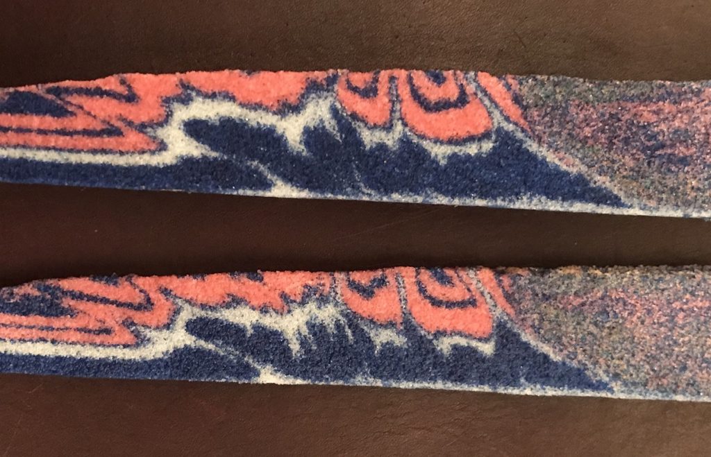
With two weak layers and localized erosion above a growing anticline, the stacking can be taken to extremes as seen in the model below.
The Sponaugle well was just one of many drilling enterprises that ended up informing interpretations of the Appalachian fold-thrust belt and many other thin-skinned sedimentary fold and thrust belts around the world. Today, structural interpretations in these settings place great emphasis on relative rock strength and anticipate zones of flat decollement faulting in shale or evaporite layers. These flats can later be deformed by subsequent faulting, creating great structural complexity. The Bolivian sub-Andes section below from Rojas Vera et al. (2019) is a good example (it is reflected to match the transport direction of images above). The anticline at the center of the image is architecturally similar to the Wills Mountain structure revealed by Sponaugle.
While Perry’s 1964 cross section would be well-received today, he was going out on a limb at the time. When the Sponaugle well was drilled, the basement-involved model for Appalachian structure was deeply entrenched. A particular champion of the model was Byron Cooper of Virginia Tech, who outlined his thoughts on Valley and Ridge structure in a 1968 paper available here. A cross section from Cooper’s paper is shown below, with several faults continuing down through sedimentary layers into basement as initially expected for the Sponaugle drilling site.
This now-disproven perspective on Appalachian fold-thrust structure centered around subsiding synclines and forces internal to the folded and faulted area, bearing some similarity to models of “wrinkle ridge” formation in lunar/planetary craters. Notably, Cooper wrote the paper containing the section above in 1968, four years after the results of the Sponaugle well were published. He chose to omit Sponaugle and other wells in Pennsylvania from the paper as they were not consistent with his favored model. Cooper’s work was based largely on outcrop observations, however, and additional drilling- and seismic-based studies from the Valley and Ridge continued to reveal details its thin-skinned architecture during the 1970s and 1980s. By 1985, thin-skinned, decollement-based structural models had been developed throughout the Valley and Ridge that are still used today and remain conceptually, stylistically, and geometrically valid.