-
Moving mountainsides: The giant quartzite landslides of the Macks Mountain area of the Virginia Blue Ridge
by Philip S. Prince
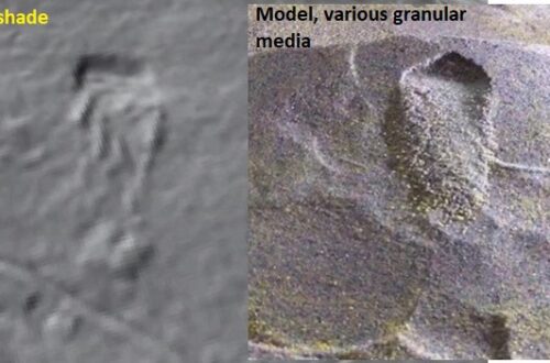
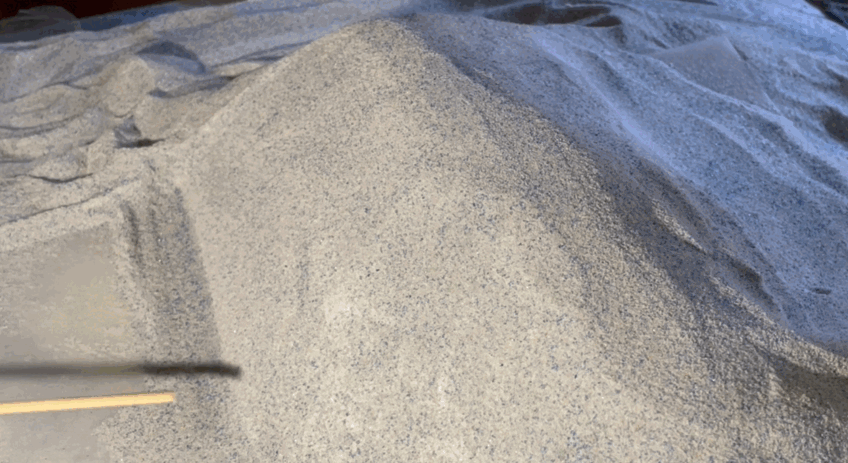
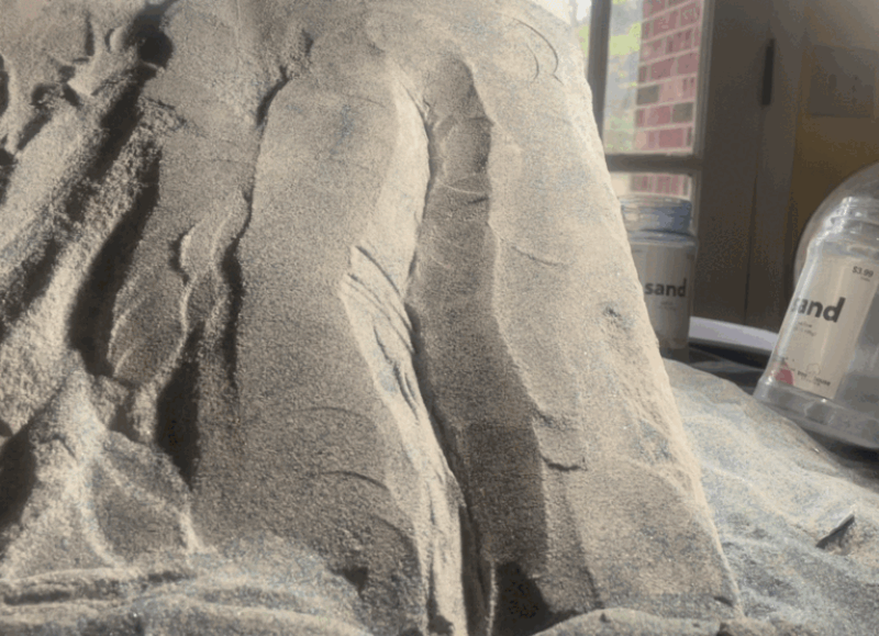
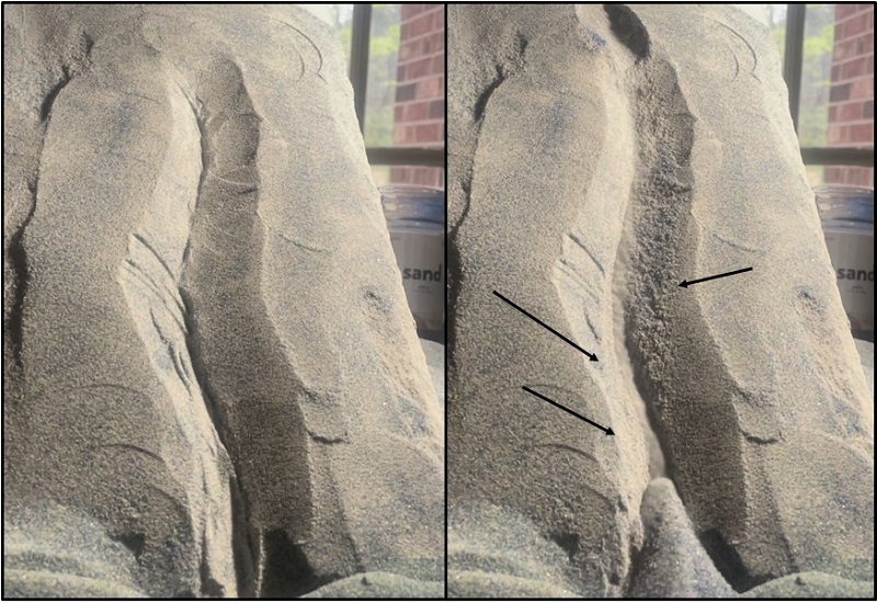
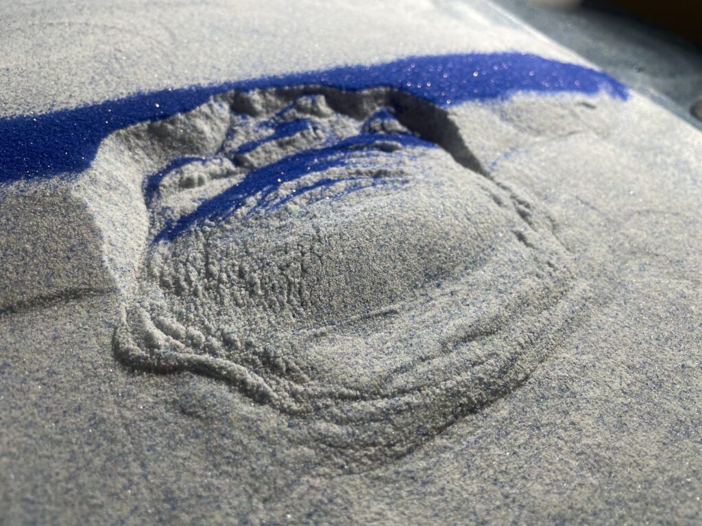
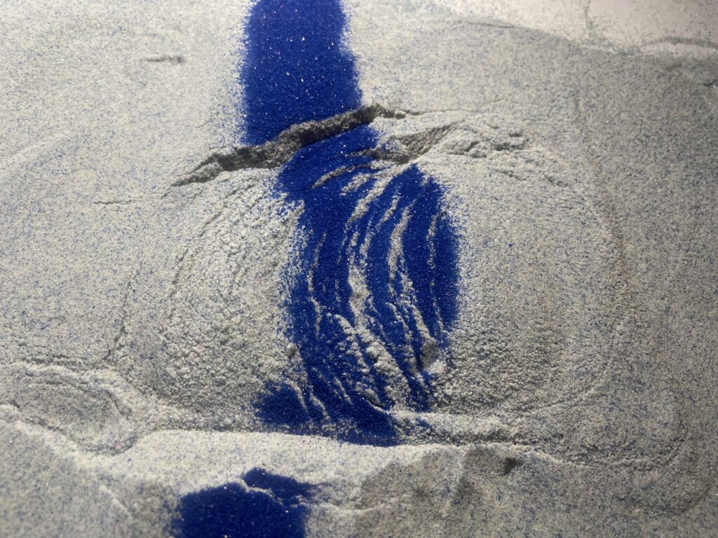
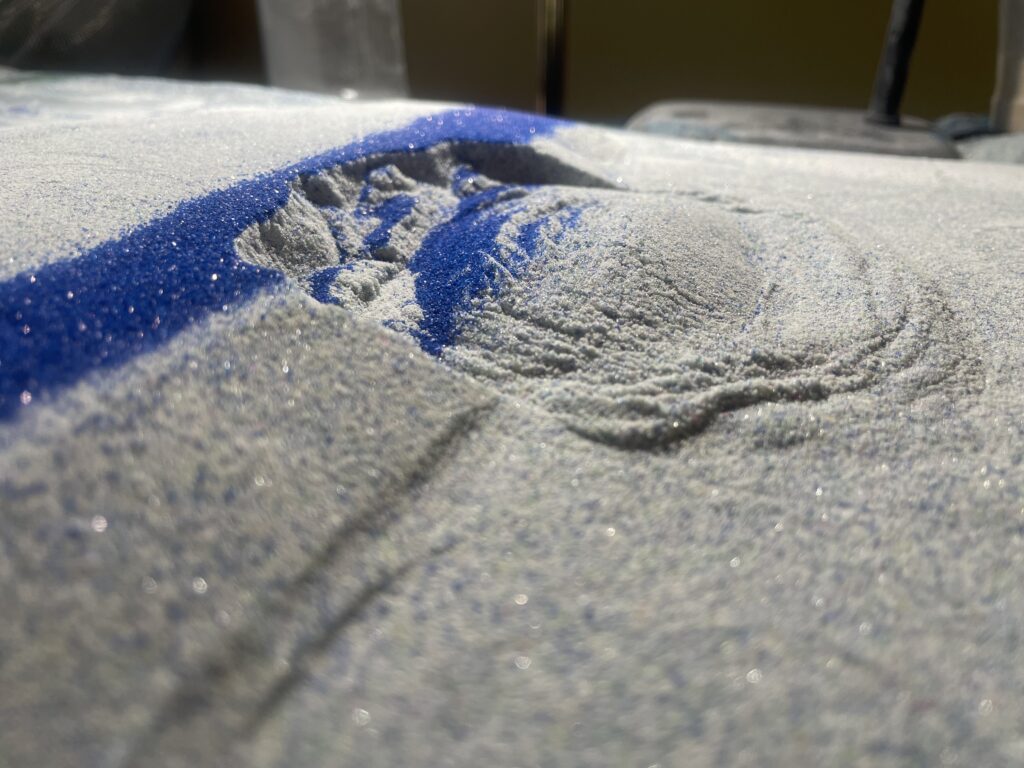
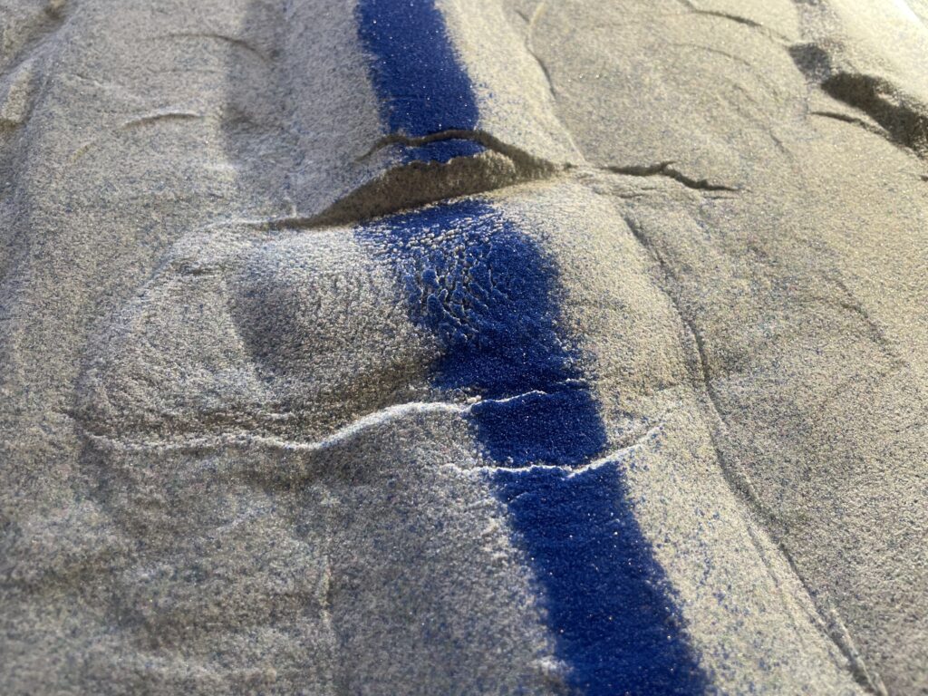
Landslides can be triggered by a variety of conditions or events. Erosional removal of the base, or toe, of a steep slope is a common cause of landsliding, sometimes creating “stop and go” landslides that move episodically when erosion carries away just enough material to create instability. After a bit of slide movement restores the shape of the slope toe, movement stops until enough material is eroded again. The model below shows what this process looks like. Scraping a tiny bit of material from the base of the slope causes an equally tiny movement of the slope. Continual scraping away of material causes the effects of small movements to add up, gradually producing a large and impressively cracked and fractured landslide mass.
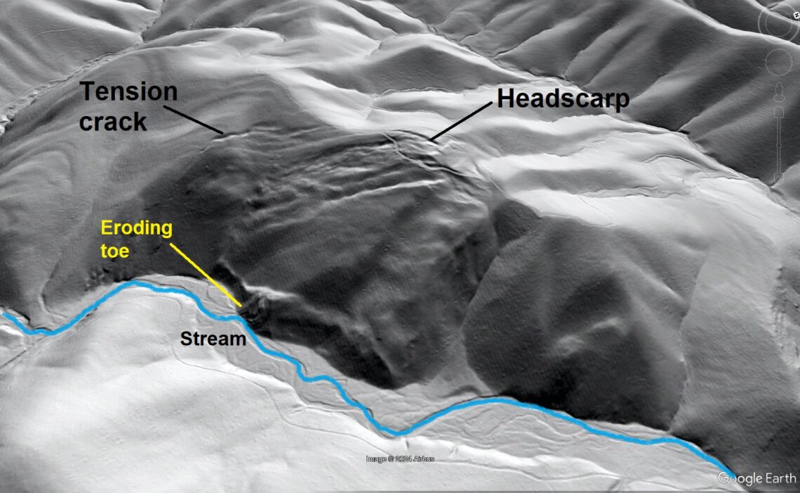
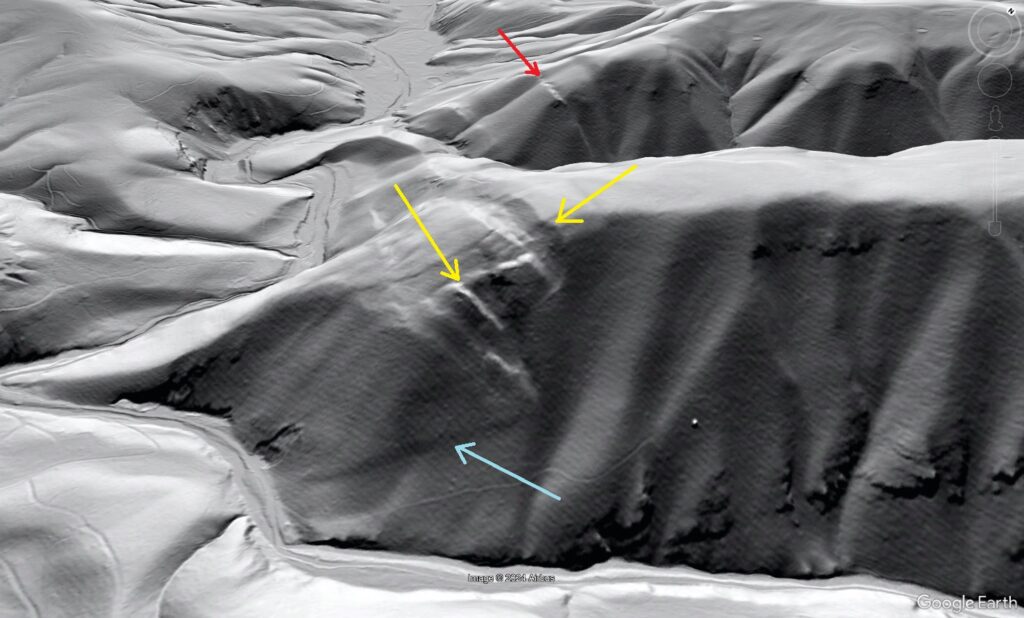
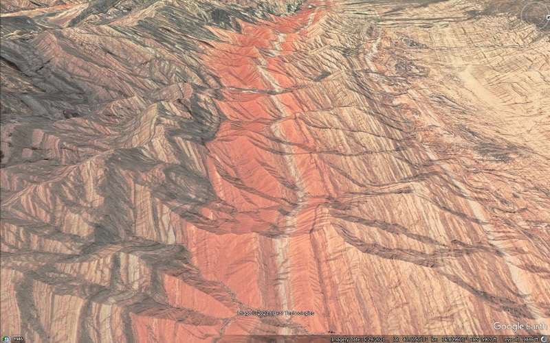
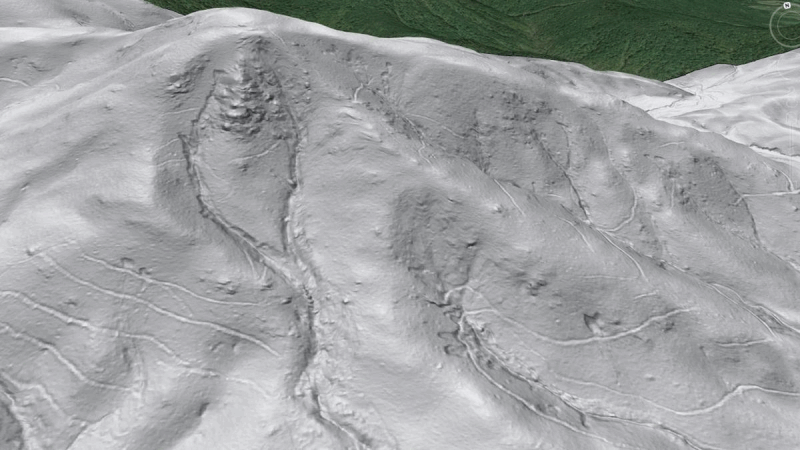
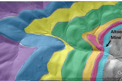
Some interesting real-world slides that appear to result from this type of ongoing erosional toe removal are found in the Macks Mountain area in the Blue Ridge of southwest Virginia (map at the end of this post). The lidar image below shows one such slide, whose appearance can be matched to the later stages of movement of the model shown above. Cracks and fissures extending from the top of the ridge are clearly visible, as is the steep, eroded toe along the stream. The slide is 2,000 ft (600 m) wide. The top of the ridge and head of the slide are about 600 ft (180 m) above the stream below.
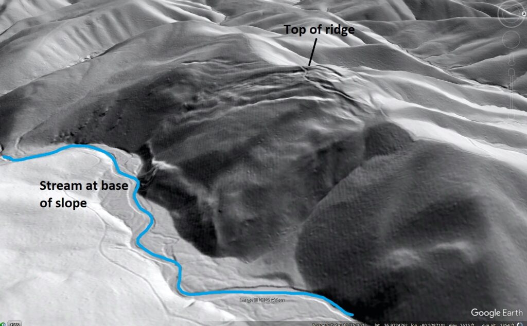
The cracks and fissures at the head of the slide along the ridge crest stand out against the normally eroding parts of the surrounding landscape. The unusually steep eroded toe of the slide, which is in deep shadow in this hillshade image, also contrasts with the even the steepest streambanks in areas unaffected by sliding. At the left side of the image, faint bedrock ribs can be seen on the land surface. These bedrock ribs indicate that layering tilts down towards the stream, favoring sliding.

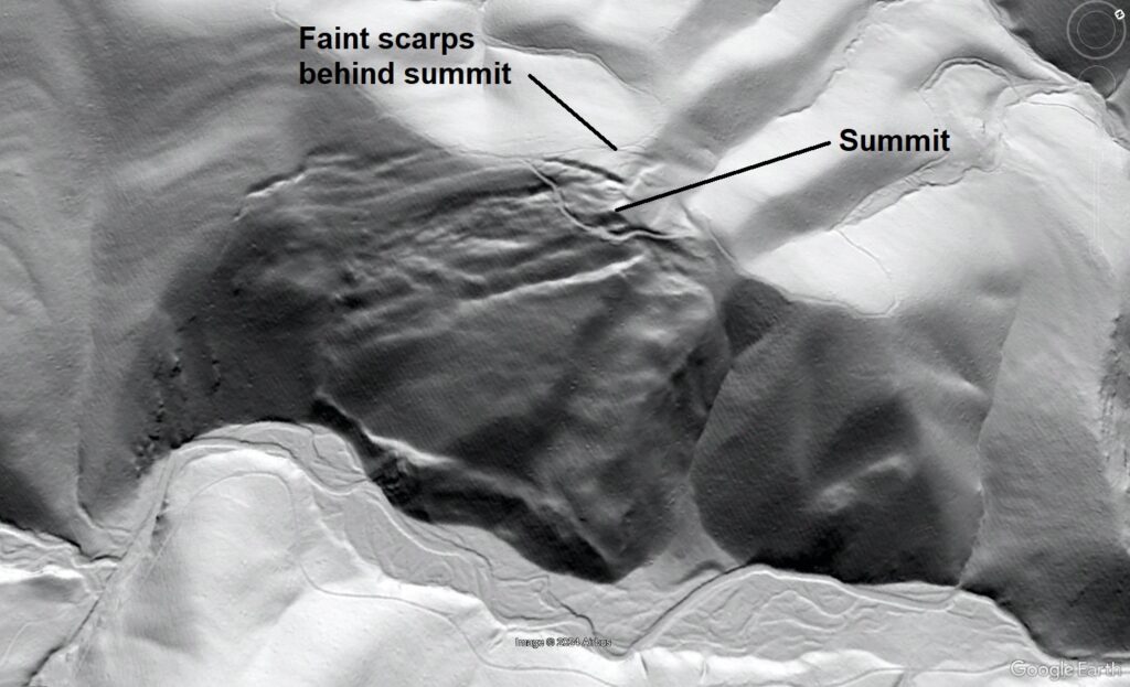
A particularly interesting detail of this slide is the presence of faint scarps or tension cracks behind the summit of the ridge with respect to the stream at the toe. In other words, the actual summit of the ridge is within the slide mass and has lowered and moved downslope just a bit. This arrangement of slide features with respect to the shape of the slope indicates that the slide is thick and is moving on a weak layer or layers deep beneath the surface of the slope.
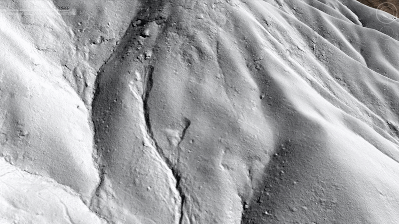
The geology of the Macks Mountain area sets the stage for numerous huge slope movements like the one shown above. Macks Mountain features rugged topography due to the presence of folded and faulted quartzite bedrock, which is quite hard and resistant to erosion, alongside weaker layers of mica-rich slate or phyllite bedrock. Slate or phyllite cannot support the slope steepness that develops due to the “armoring” effect of quartzite layers, leading to big landslides that slowly feed rock into the eroding streams below. Lidar imagery makes the slides easy to see, but their size and subtlety would make them less than obvious to a ground observer. The example shown below features the characteristics seen in the previous slide.
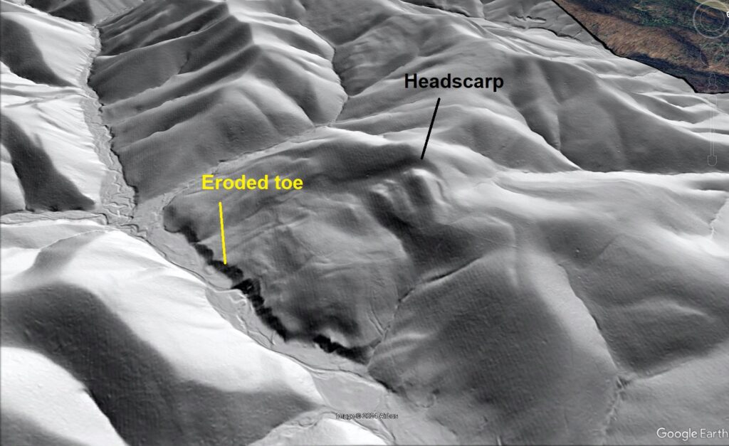
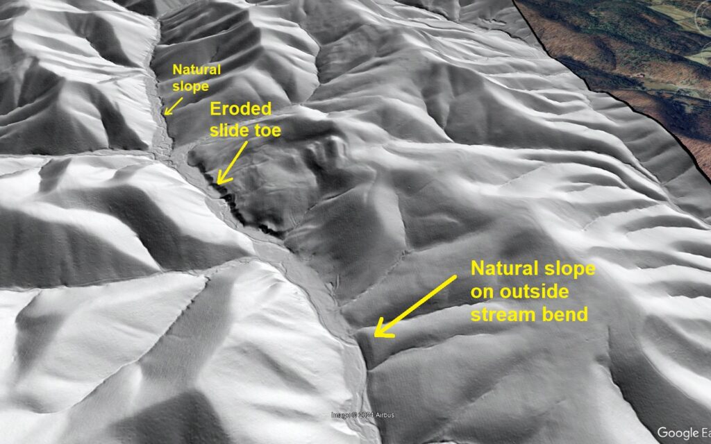
This slide is a bit less crisp and sharp, suggesting it might be a bit older or be in a longer period of suspended movement. Even so, the steep, eroded toe and blocky, lumpy topography below the headscarp contrast nicely with the surrounding erosional topography. The eroded toe area is particularly distinct, and is notably different from even the steepest streambanks in areas not affected by sliding, as seen below. This toe steepness suggests some slide movement is recent enough that the toe has not yet returned to an appearance more like the undisturbed landscape.
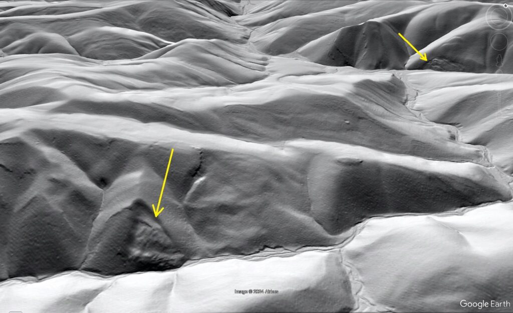
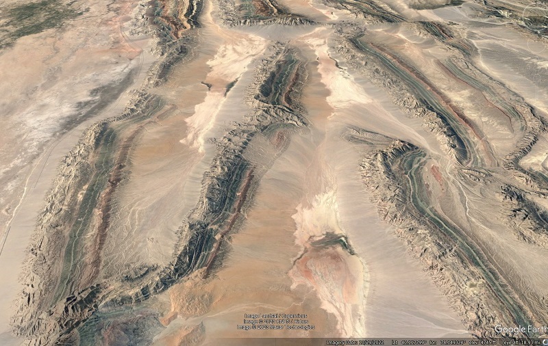
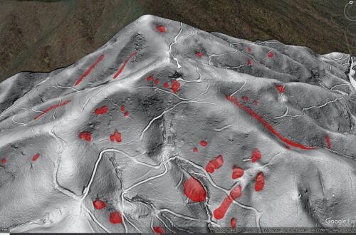
Bedrock-involved landslides like these come in a variety of sizes in the Macks Mountain area. Some smaller slides appear to have destabilized larger areas of the slope, possibly setting the stage for future movement of larger areas. The small slides indicated by yellow arrows below are about 1/4 the size of the first slide in the post, but they have developed for the same geologic reasons.
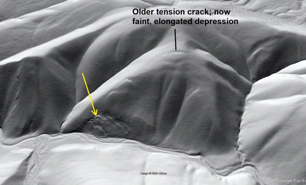
The slide in the background of the image above appears related to older tension cracks well upslope of the crisply defined slides. Now a faint, elongated depression, the upper tension crack suggests that a huge portion of the slope once experienced a tiny amount of movement, and might shift again in the future.
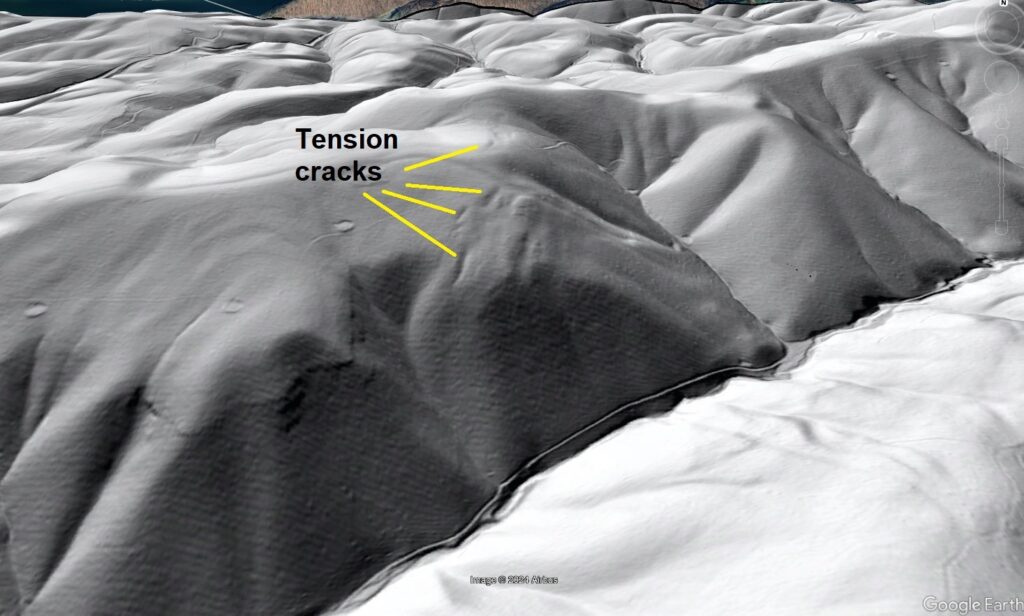
Other old tension crack sets do not have any obvious recent slides associated with them. These cracks also suggest that slopes in the Macks Mountain area exist at the threshold of movement, possibly due to stream incision and relief production associated with the downcutting of the nearby New River. The tension cracks shown below are similar to the example above, though more numerous. A road grade and stream are present at the base of the slope, though no smaller slides are visible. The tension cracks would appear as subtle depressions in the forest today, as soil development has dulled their outlines.
Near this group of old tension cracks, two unusual topographic features are likely the result of the largest and thickest slope movements in the area, although their unusual appearance makes interpretation more difficult. These possible slides are shown below.
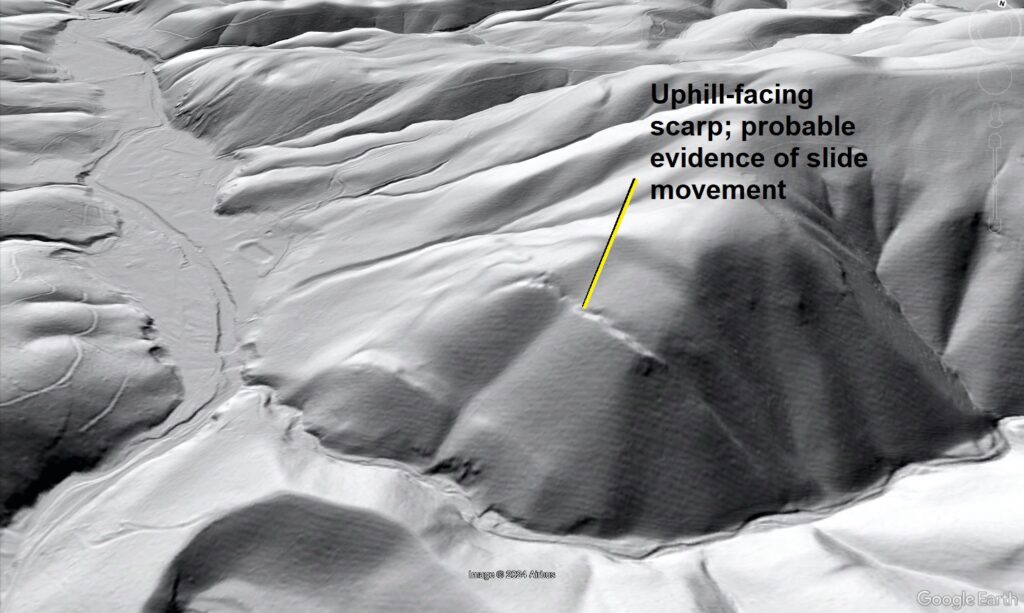
In both images, yellow arrows indicate probable scarps that are significant to a landslide interpretation. In the image above, the light blue arrow shows a likely toe bulge related to faint downslope movement. The red arrow in the background indicates the position of the uphill-facing scarp in the previous image. These features lack the ease of interpretation of the other slides shown, but their features are effectively impossible to explain without slope movement. Uphill-facing scarps and the associated localized surface depressions are very significant. “Typical” sinkholes related to bedrock dissolution do not form in this type of rock, so any surface depression results from a physical gap due to slope movement or excavation by humans. The model below shows uphill-facing scarp development, along with localized sinking of the model surface.
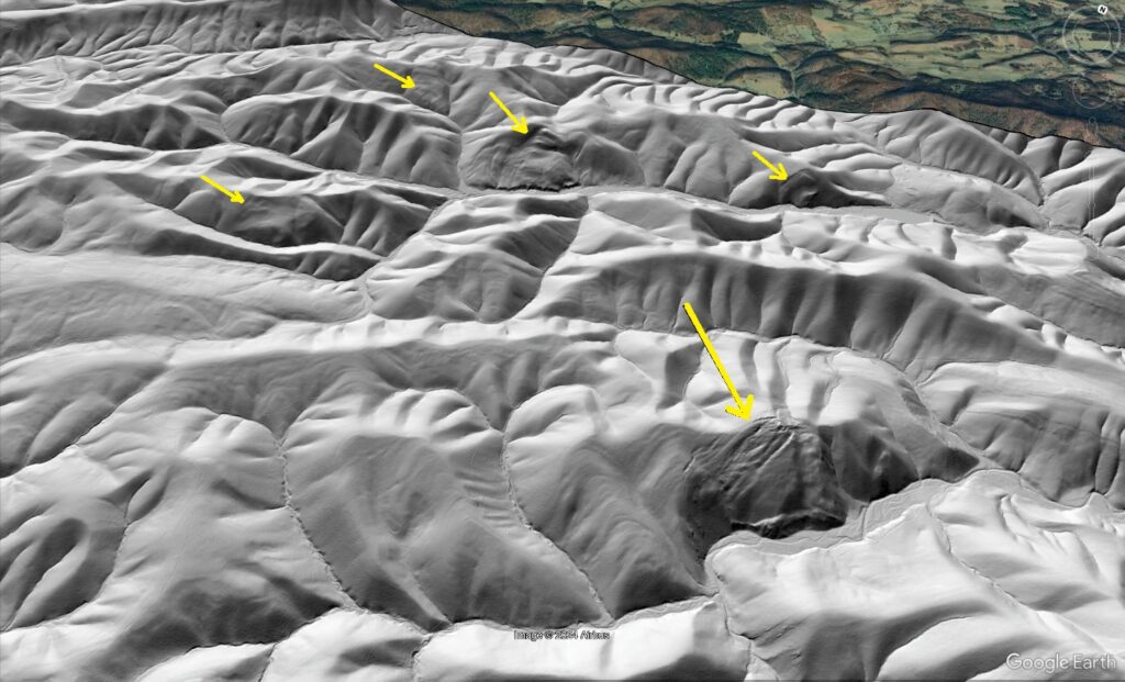
The big “mystery” features do not resemble surface excavation in any way. They are very large, oddly shaped, and have formed in areas with no access roads for the equipment and personnel necessary to remove such large masses of rock. Due to the prevalence of large-scale bedrock landsliding in the area, the “mystery” features can reasonably be interpreted as large slope movements. A zoomed-out view of the surrounding area shows that landslides aren’t hard to find in amongst the ridges of Macks Mountain due to the bedrock character, slope steepness, and likely history of relief production in the area. Yellow arrow point out slides in the image below, which is a nice practice image for pattern recognition in lidar interpretation.
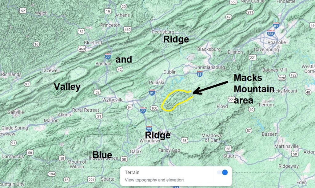
Big bedrock landslides are a common topic on this blog, as they are fundamental feature of many mountain landscapes in southwest Virginia. The most well-known slides occur in the Valley and Ridge, where tilted sandstone layers slide on weak shale layers. Macks Mountain is underlain by metamorphic rocks of the Blue Ridge province, but quartzite and phyllite are just slightly “cooked” sandstone and shale, respectively. Quartzite and phyllite retain the extreme mechanical contrasts of sandstone and shale and behave accordingly in the landscape. The relative locations of the Macks Mountain area and the Valley and Ridge are shown below.
A particularly interesting aspect of Macks Mountain slopes is that none of the slides appear to exhibit large-scale, rapid movement that would be particularly dangerous to people in the area. Topographic evidence suggests the slides just creep along, and may see suspension of movement for very long periods. While they don’t threaten people living nearby, engineering projects would need to avoid the slides. As stream erosion appears to be a driver for their movement, excavation of the toe of slide to build a road or any sort of structure in a stream valley would likely lead to movement. Projects like pipeline construction also need to consider this type of slide, as even slight movement can have catastrophic effects should the movement rupture a pipeline. Fortunately, high-quality lidar imagery makes big landslides like these easy to see in the landscape, supporting good decisions with regard to land use and development.
You May Also Like
Real sandbox model meets “numerical sandbox” model…an interesting comparison of dry granular media and discrete element simulation
The geology lab cross-cutting relationships exercise as a sandbox model
Formation of anticlines and synclines above sandbox model normal faults with changing dip
-
Formation of anticlines and synclines above sandbox model normal faults with changing dip
by Philip S. Prince
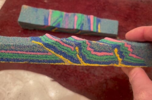
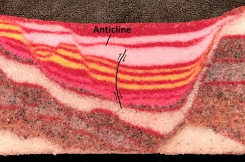
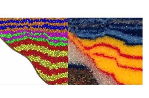
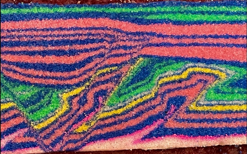
While Earth’s most dramatic geologic fold structures result from compressional deformation, extensional deformation can also produce closed, upright folds–in both the real world and in physical models. Extensional anticlines (particularly when upright and generally unfaulted) are always more subtle than their compressional cousins, but extensional synclines can be very tight with very steep limbs, particularly when pronounced “space problems” develop in the fold hinge. The image below compares extensional folding (top) with compressional folding in two sandbox models made from mechanically similar sandpacks deformed in different ways.
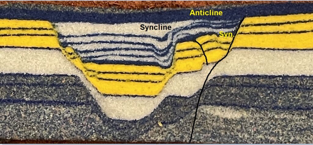
Extensional folding seems to get less hype in the world of geology visuals, but extensional fold structures are extremely significant in the world of hydrocarbon exploration and subsurface storage. Analog models readily produce illustrative extensional folds that develop for the same reasons as real-world structures (see the end of the post). The image below shows a suite of sandbox models I made with the development of extensional folding in mind (or lack of folding, in the top model) . With a close look, subtle anticlines, and one much less subtle syncline, are visible in all but the top model. There’s a reason for this, discussed below.
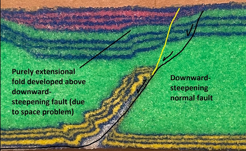
All of the folding developed in the models is some sort of expression of forced, fault-bend folding, which develops when the hanging wall makes geometric adjustments to match changing footwall shape. “Changing footwall shape” basically means changes in fault dip. As a hanging wall block moves across a locally flattening or steepening fault, it must constantly change its shape to prevent void development and match the footwall shape. This concept has been illustrated and GIF’d a few times on this blog page already, with the GIF below being my newest and simplest expression of the idea.
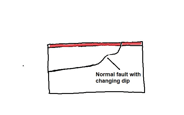
In the first frame that shows hanging wall movement, voids or open spaces develop at the steep parts of the fault. Such void development is impossible at tectonic scales (miles/kilometers of rock), with the hanging wall steadily collapsing as it moves across dip changes to maintain contact with the underlying fault plane/footwall. Fault flattening forces collapse and stretching in the hanging wall, while a zone of fault steepening after a flat forces a space problem that may result in development of an accommodation fault with local reverse-sense movement. You can see examples of these accommodation faults in the second image in the post, particularly in the orange model at the bottom.
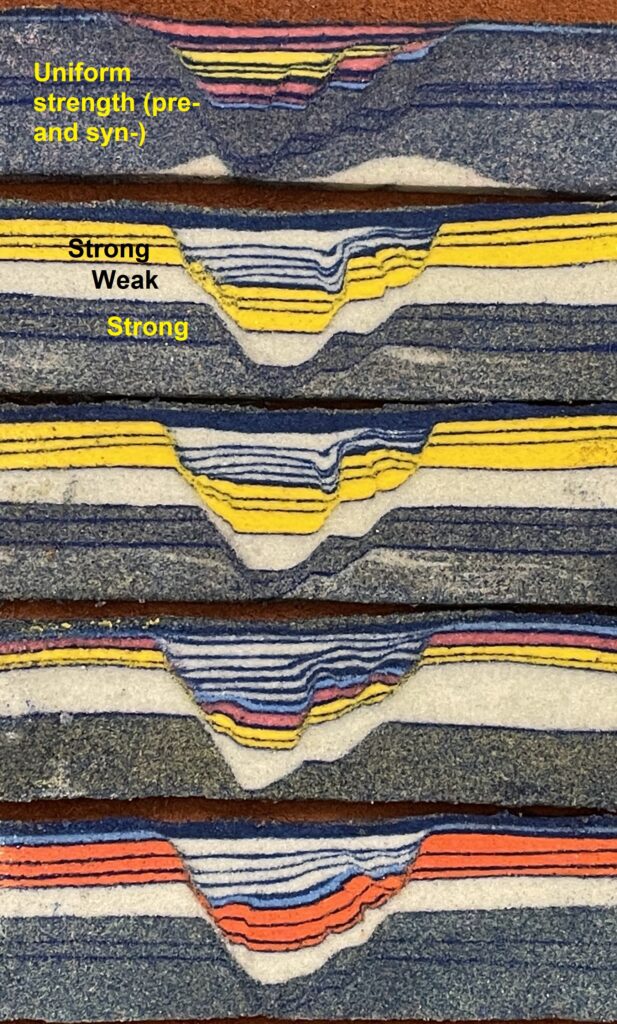
Fundamentally, change in fault dip is a key driver of folding in the extensional regime. Since granular media with different internal frictional behavior produce different model fault angles, extensional folding can be induced by constructing models with different strengths at different depths. No rigid, non-granular blocks are necessary. Mechanical contrast and few degrees of difference in fault dip is adequate, as shown below.
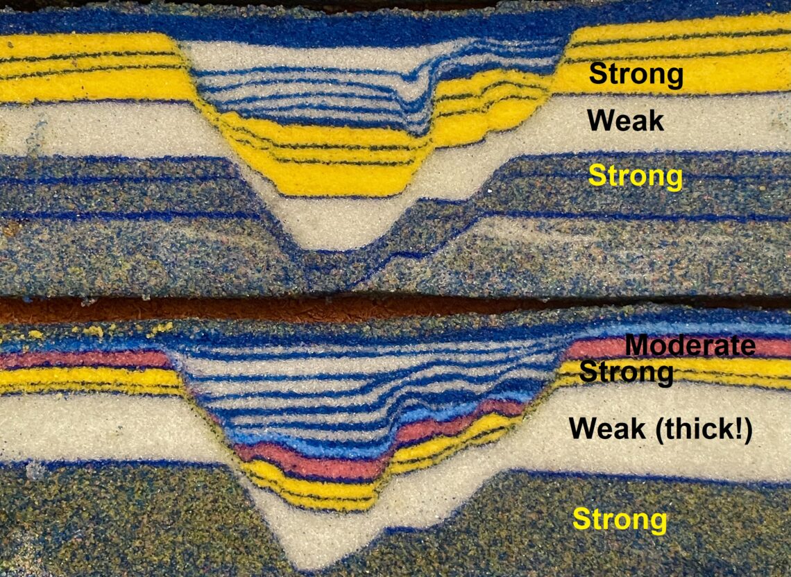
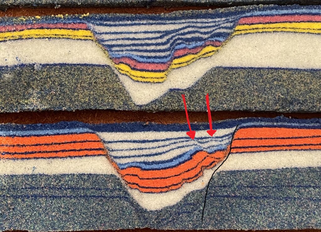
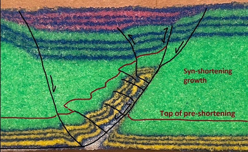
Analog models using contrasting materials (here, white glass microbeads, yellow and orange dolomite sand, and pink quartz sand) produce structures that are a direct reflection of mechanical stratigraphy. The upper model in the image below uses a thick, strong section (yellow) above a weak layer to produce a distinct structural style, including an impressively tight syncline in the growth section. The lower model uses a combination of weaker strata above a thick, weak horizon in the pre-extension section to create a broad zone of undulating folding in the white/blue growth sequence. Model setup and deformation was effectively identical; only the mechanical stratigraphies are different.

The orange sand in the lower model of the following image has mechanical properties somewhere between the yellow and pink sands in the other models. The resulting structural style is also transitional, lacking both the extreme syncline formation of the thick yellow model and the broad, undulating zone in the model containing pink sand. Instead, two anticlines (indicated by red arrows) formed in the growth section above the zone of fault (black line) dip decrease within the weak white layer. Note the little reverse sense-fault (see the GIF) and the upright anticline against the left side basin-bounding fault.
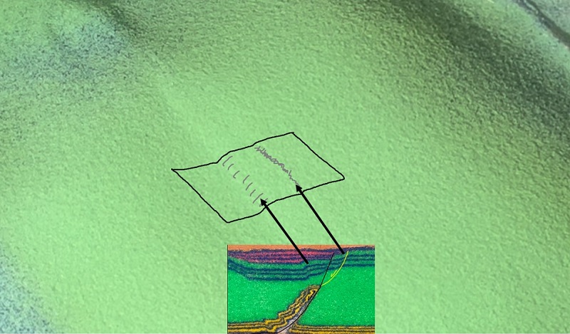
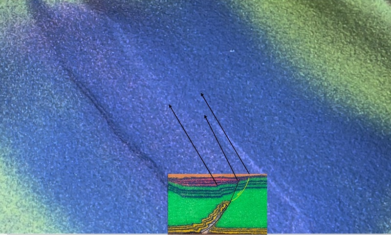
I have never had success in developing this sort of extensional folding clearly against a clear glass sidewall, but the process is visible when the models are viewed from the top. The images below indicate the position of cross section features on plan view images of the deforming models.
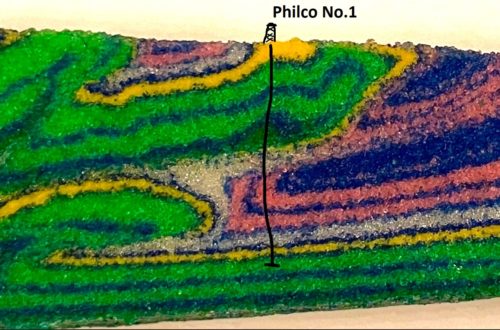
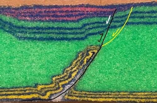
These are simple, direct extension models; they use a moving baseplate that does not stretch to create more distributed extension and a “domino block” structural style. Despite their simple setup, the models do create structures that are reminiscent of well-known, real-world extensional anticlines, as shown below. Note the association between the position of the real-world hanging wall anticline below and the flattening of its associated normal fault. The white arrow in the model image indicates the crest of the main hanging wall anticline. “Real-world” image source here…
I am very much a fold-thrust belt kind of guy, but extensional structure is always interesting to consider. I think the elegantly simple relationship between fault dip and hanging wall deformation is one of the most classic and illustratable concepts in all of geology, which probably explains why there are a number of extensional fold posts on this blog!
-
The geology lab cross-cutting relationships exercise as a sandbox model
By Philip S. Prince
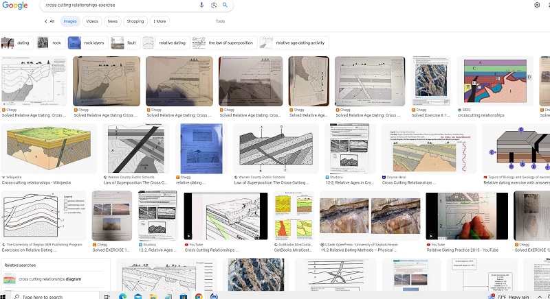
If you have studied geology in recent decades, you have probably encountered a cross-cutting relationships exercise, particularly in a lab class. These exercises are an important part of establishing the order in which particular events occurred, and thus understanding which structural and stratigraphic feature may impact–or be impacted by–other features. Most cross-cutting relationships exercises features deformed sedimentary layers, angular unconformities, igneous intrusions, and faulting that offsets pre-existing elements of the exercise. Give “cross-cutting relationships exercise” a Google search, and you’ll find no shortage of examples:
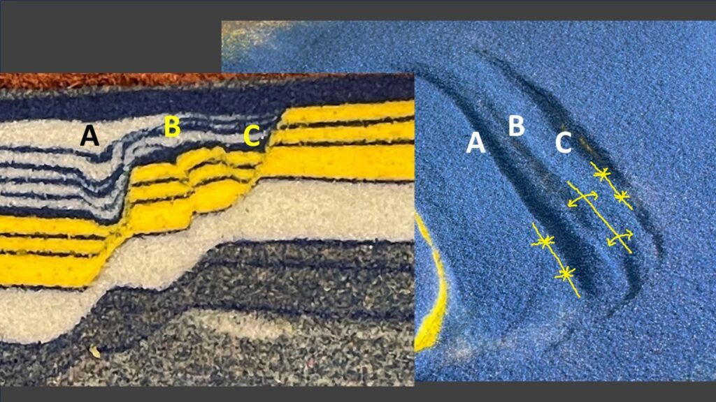
I thought it would be interesting to turn this ubiquitous classroom activity into a real-life analog model. Igneous intrusion is a bit beyond my scope, but deformation, erosion/unconformities, and subsequent deformation are easily achieved in a 3-D “table top” model with overlapping, movable base plates. The image below shows a portion of the model I produced. This first look is a zoomed-in detail that is reminiscent of the format of the exercise drawings.
I admit that the color scheme is grotesque, but I purposely wanted to reduce extreme contrasts so that the appearance is initially a bit confusing and requires that angular relationships and offsets be carefully studied (the colors may be especially bad for folks with red-green issues). All of the events that affected the model can be observed in this detail. The events are listed later in the post, but give this image a look first to see if you can figure out what happened and in what order.
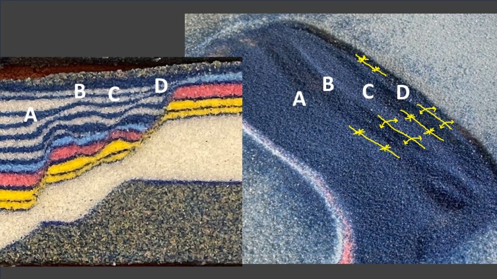
The full model is shown below.
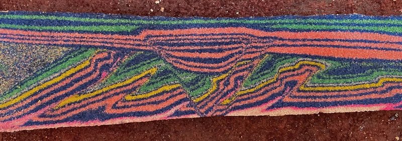
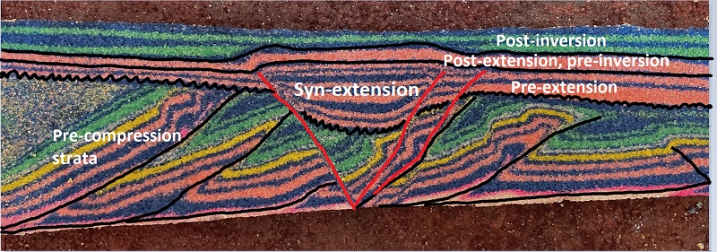
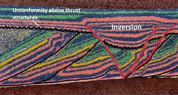
When the entirety of the model is seen, numerous sequential thrust structures are easily visible. The top of the thrust structure at far left terminates suddenly against nearly flat-lying layers above it. Upon closer inspection, other thrust structures can be seen to terminate at an angle against the overlying blue and pink layers. This termination is an angular unconformity, meaning an erosional event post-dates thrust faulting and associated folding. The squiggly black line in the annotated image below shows the angular unconformity.
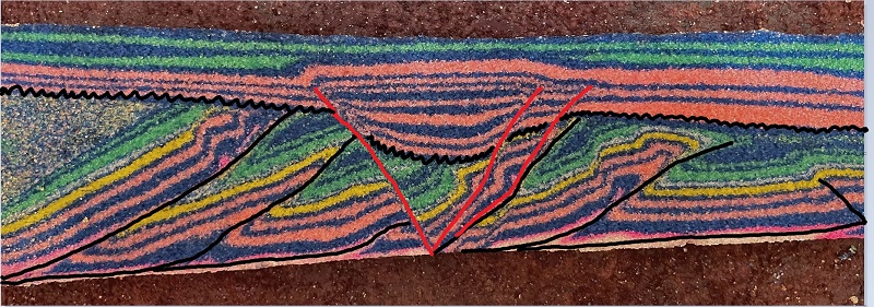
In the middle of the model, the angular unconformity is offset and down-dropped by normal faults. This normal faulting post-dates the angular unconformity. Several pink and blue layers present above the down-dropped portion of the unconformity are not present elsewhere in the model; these are growth strata that were deposited in the extensional basin that developed above the normal faults. The thick package of strata is no longer in a structurally low basin, however, as it has been inverted after normal faulting and basin filling. The uppermost green layers lap onto the uplifted, inverted basin, with an undeformed green layer covering the basin and post-dating inversion.
Which beds pre- or post-date extension and inversion is not immediately obvious, so the annotated image below labels these intervals.
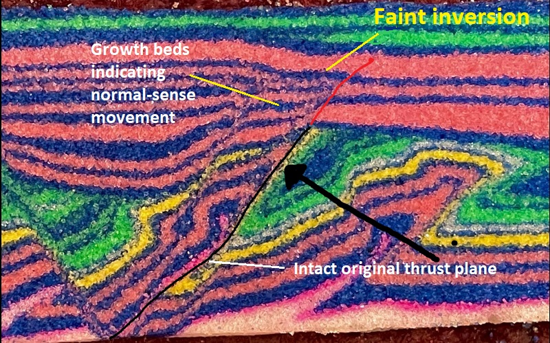
A notable detail of inversion in the model is the reactivation of normal faults during the inversion process. Inversion was produced by highly oblique movement, with the portion of the model on the right side of the basin moving towards the observer during the final deformation sequence. Oblique movement permits reactivation of existing normal faults, which are too steep to reactivate under direct compression in a model using these analog materials.
An even more interesting detail is that the fault bounding the extensional basin on its right edge was initially a thrust fault that back-rotated as more thrust structures developed after its formation. During extension, the back-rotated thrust reactivated as a normal fault due to its steeper dip. During inversion, it reactivated yet again, though only slightly. The fault thus experienced thrust, normal, and reverse/inversion movement during the various phases of model development. This intriguing structure is detailed below.
The overall “order of operations” is:
- Deposit white, pink/blue, yellow, green/blue sequence
- Compression and thrust belt development affecting layers from step 1.
- Post-thrusting erosion of compressional structures.
- Deposit two pink/blue layers atop erosional surface; angular unconformity.
- Extension and normal faulting; deposit several pink/blue sets in growing basin. (Normal-sense thrust reactivation).
- Deposit one thick pink/blue horizon atop entire model, including filled basin.
- Inversion of basin, deforming the thick pink layer deposited in 6 as well as the basin fill. (Reverse-sense reactivation of thrust/normal fault).
- Deposit green/blue sets.
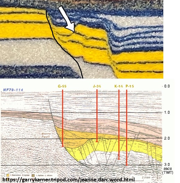
Classroom exercises of this type are a key step in learning to see geologic structural relationships as an expression of various phases of movement and change. While the exercises are specifically produced as simplified classroom examples that are a bit out of context, the interactions they (and the model) show are very much real-world features. Compare the conceptual diagram below depicting a portion of the Pannonian Basin of Hungary with the model. The image was sourced here; I reflected it to match the sandbox model’s thrust orientation. Note the scale bars; this diagram depicts kilometer-scale features that are vertically exaggerated.
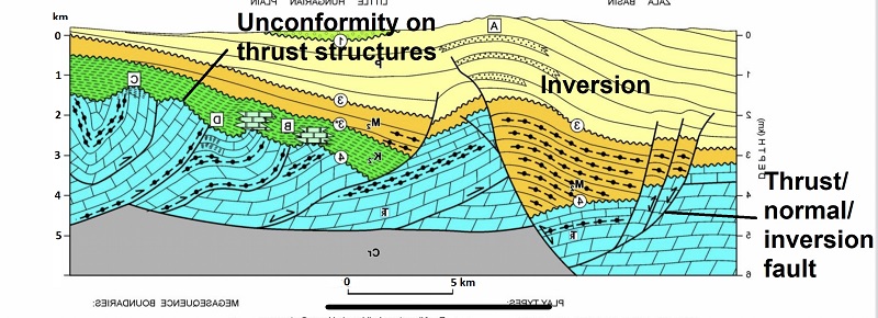
The features shown in the diagram generally match the idea of the model.
Interestingly, I didn’t intend the model to match the Pannonian example. The model came first, and I wanted to seek out a real-world example. I knew the Pannonian Basin was an example of a setting where extension had caused pre-existing thrust belts to subside and be buried, so I went looking for a basic visual to depict interpretations of this structural style. I wasn’t aware of inversion in the area; this was a nice surprise in terms of matching a diagram to the model!
The compression-extension-inversion sequence depicted in the Pannonian example certainly happens in other settings where subduction zone-related compression transitions to extension due to slab rollback. I admit I don’t know exactly what triggers the return of compression and associated inversion, and I would absolutely love to know the explanation! Numerous other cross-cutting tectonic events are possible as well, such as Mesozoic, continental break-up rifting developing extensional basins in the Paleozoic compressional Appalachians. The Mesozoic event introduced plentiful diabase dikes into the multiply deformed rock mass. The modern-day Appalachian stress field is characterized by North American margin-parallel compression, which might be appropriate to start inverting the basins. A geologist working in the Appalachian Piedmont would need to consider all of these events and factors in order to fully understand the Piedmont surface and subsurface, providing another example of how the good old cross-cutting relationships exercise has real relevance.
-
A sandbox model of China’s “other” Rainbow Mountains that fits in the palm of your hand
by Philip S. Prince
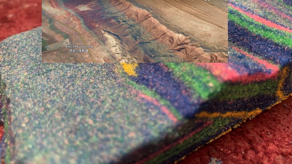
If you spend any time on the internet, you’ve probably seen an image of China’s Zhangye Danxia Landform, also known as the “Rainbow Mountains.” While these colorful landforms get most of the hype, China hosts another, arguably more impressive, zone of colorful, tilted sedimentary layer mountains–the Keping fold-and-thrust belt. Located at the northern edge of the Tarim Basin, the Keping showcases elongated ranges of pink, green, purple, and tan mountains that stretch for 10’s of kilometers and are readily seen from Google Earth. The two images below show details of some of these ranges, where distinctly colored sedimentary layers are easily visible.
The following image shows a zoomed-out view, with the color patterns still visible in each of the elongated ridges/ranges.
The beauty of landforms like these offers a nice (and seldom exploited) opportunity to connect surface landforms with underlying geologic structure. The lack of vegetation and varied color of the sedimentary layers clearly illustrates that tilted layers underlie the Earth’s surface and form the mountain ranges, but the nature of the process of tilting and erosional exposure, as well as what the layers do far below the surface, is less obvious. A basic analog “sandbox” model using colored sand layers can capture these overall processes and put the large, real-life landforms into a more understandable context. This “scaling down” of size and time is useful, as a modern-day observer only sees a localized snapshot of a large-scale, millions-of-years process. I made the sandbox model below in a couple of hours to shrink and fast-forward the development of the Keping fold-thrust belt. The layer sequence was specifically chosen to match the stratigraphy seen on the Keping mountain ridges.
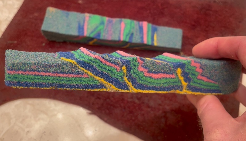
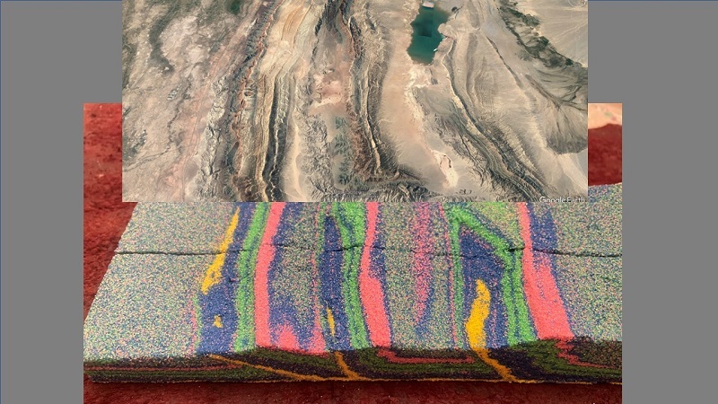
The model was not produced in the solid, hold-in-your hand condition as seen above–more on that below. It was made by shortening a sequence of loose, dry sand layers against a fixed backstop. The result was thrust faulting and associated folding/tilting of the layer sequence, with uplift of the tilted layers as they moved up thrust ramps. A bit of sand was carefully scraped away from the uplifted areas to replicate local erosion above the thrust faults. The real Keping fold-thrust belt essentially formed in the same way; a sequence of sedimentary layers was shortened against a thick, mechanically stronger mountain belt core by movement of the underlying tectonic plates. The image below shows a top view of the model below a Google Earth view of the real fold-thrust belt. In both the real fold-thrust belt and the model, thrust faults upturn and repeat the layer sequence three times.
The GIF below shows an abbreviated version of the model setup. Deposition of layers, followed by shortening and erosion, expose the buried colored layers where they tilt and uplift above thrust faults. While this is a highly simplified model, it illustrates the basic steps in the formation of the Keping fold-thrust belt (a millions-of-years process!) as it is seen today.

The model was soaked with gelatin and carved slightly before it completely dried to produce the final “topography”; the crisp ridges in the final, solid model cannot be produced in the loose, dry sand before gelling for preservation. I tried to scale the overall thickness and length of the layer pack, along with individual layer thicknesses and colors, to match up closely to parts of the real Keping fold-thrust belt. As seen below, it worked well. The small panel of Google Earth imagery grafts nicely onto the model.
Loose, dry sand is a good analog for rock in the upper few kilometers (generally less than 12km or so) of Earth’s crust due to its internal frictional strength/behavior and lack of cohesion. As a result, structures made in sand layers at the centimeter scale actually do reflect geometric characteristics of kilometer-scale geologic structures. The Keping fold-thrust belt is fairly simple in that a single, basal detachment largely controls its structure, so it is readily replicated with a basic model.
A notable detail of the final “carved” model is the size of the mountain topography. It is not particularly large compared to overall thickness of the fold-thrust belt and the size or depth of the thrust structures. This relationship is seen in all of Earth’s sedimentary fold-thrust belts; surface topography is always significantly smaller than the scale of the subsurface structures that support it. The real Keping is up to 10 kilometers thick; the mountain ranges developed on the thrust sheets rise about 1.5 kilometers above the surrounding landscape. The “mountains” carved onto the model are actually a bit too big. If you can read backwards, the vertical scale on the cross section below will give you a sense of the size/depth of the real Keping system.
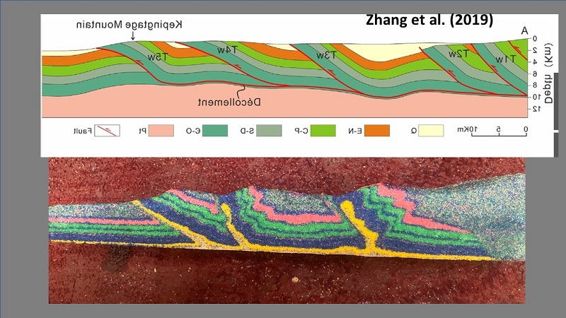
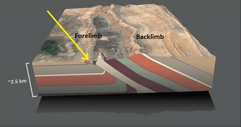
I drafted the generalized block diagram below to give an idea of basic structure beneath the real outermost Keping ridge (the Kepingtage Mountain, I believe), with indication of physical size and depth. It is based on both the cross section above and details of the sandbox model. Note the scale bar at left. The sequence of layers that is thrust faulted to form the Keping fold-thrust system changes in thickness along its length, so the thicknesses don’t quite match the published cross section above.
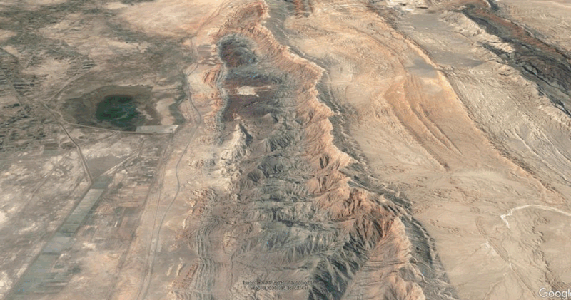
The small model, like many analogue models, goes beyond capturing the overall details of the real structure–many smaller, more subtle details are also reproduced. Sharply upturned pink and green layers (yellow arrows) are visible on the forelimbs of the real structure shown in the GIF as well as in the model. These upturned layers are cut off by the main, frontal thrust fault below the surface…and probably not very far below it. They are also atypically thin and distorted due to their forelimb location, immediately above the thrust.
Analog models are great to look at, but it is important to remember that they develop their structural architecture due to the same physical principles that guide the formation of full-size, kilometer scale geologic systems. The defined geometries seen in analog models are very much present at the kilometer scale, where they are just too big–and buried–for an observer to appreciate. Settings like the Keping fold-thrust belt offer a chance to see clearly expressed evidence of this defined geometry. This style of pattern recognition can then be applied elsewhere, such as in settings where surface vegetation obscures a clear view of rock outcrop patterns.
-
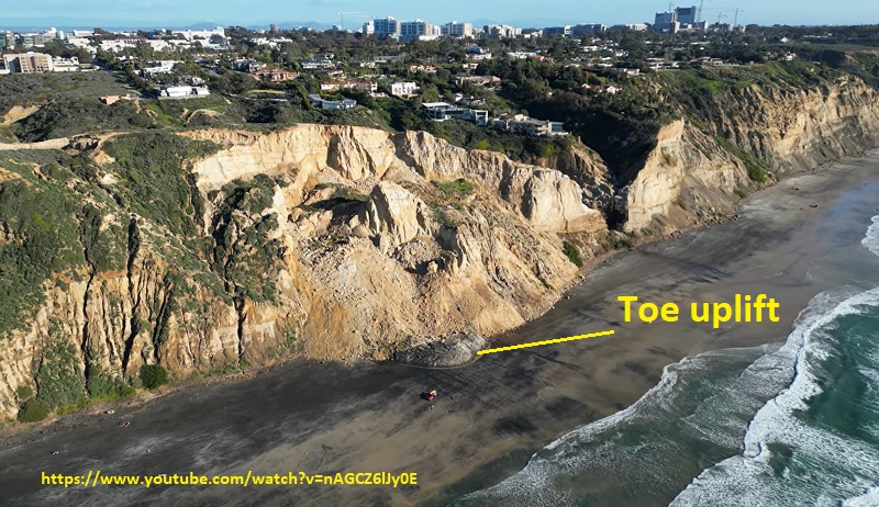
The Blacks Beach landslide: Why did part of the beach rise as the cliffside slid down?
by Philip S. Prince
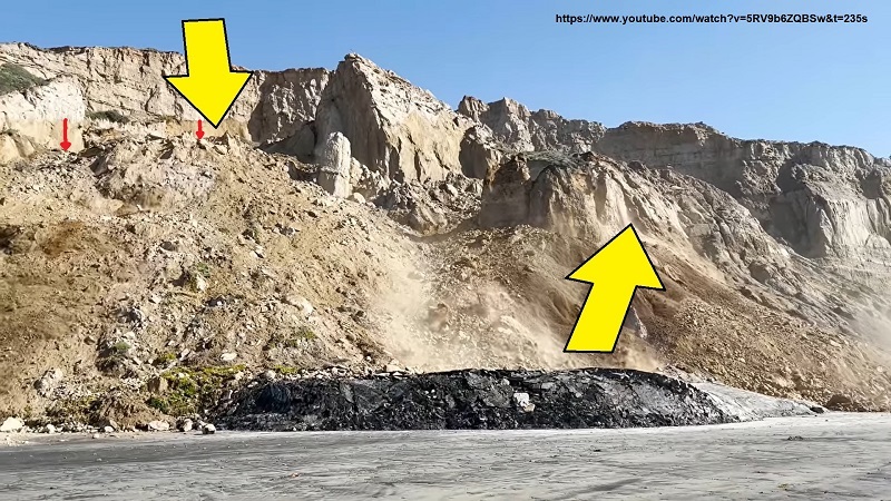
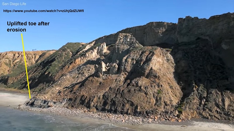
The January 20, 2023, landslide at Blacks Beach near La Jolla, California, dramatically uplifted a small portion of the beach during the slide’s movement. Filmmaker Kent Ameneyro captured the uplift sequence in great detail in the YouTube video linked here. From ground level, the uplift is very dramatic, particularly against the backdrop of the downward displacement of the steep slope above it. The image below is a screenshot from the Ameneyro video, with large yellow arrows indicating the general movement. The small red arrows up the cliff indicate visible offset as the slide block moves.
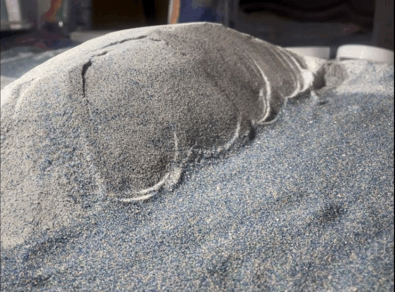
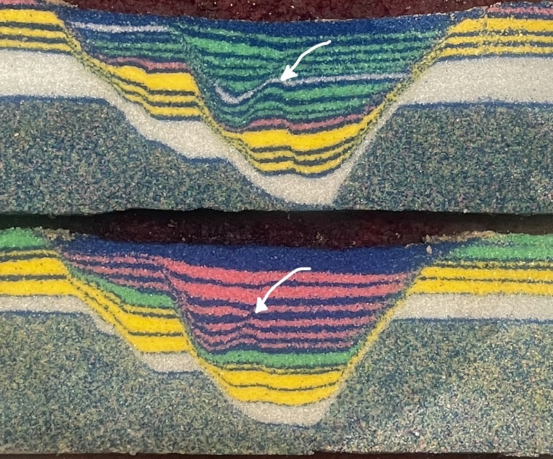
The beach uplift produces an understandable reaction from onlookers, and many of the early comments on the YouTube video focused on why it occurred. In this case, the uplift is directly related to what is below the land surface–weak mudstone layers that provide a nice slide plane underneath the base of the slope and the beach. I made the model shown below about a year ago to illustrate this slope failure scenario, and Blacks Beach provides a nice opportunity to relate it to a real-world slide that happened to be filmed (the model wasn’t!). The weak layer and its depth below the model surface allowed failure of the sand layers to extend beyond the base of the slope, driving the the toe of the slide up as the head of the slide sank down to produce a headscarp and sag. The downward motion at the head of the slide thus drives the upward motion of the toe.
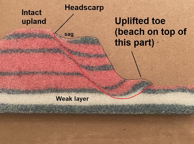
The image below uses arrows to illustrate this general motion.
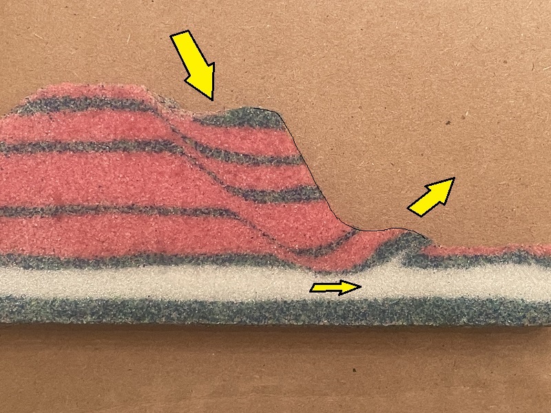
The model in the GIF below portrays this process from the landscape view. If the model were cut away like the one above, a similar pattern would be present. Again, a weak layer well below the base of the slope causes the slope and a portion of its base to move together, with downward motion of the slope causing outward and upward motion of the toe. Movement of the darker sand layers beyond the base of the slope starts as soon as the top of the slide begins to move downward, showing that the areas are linked along the same sliding surface. The light material of the slope isn’t really pushing or “bulldozing” the dark sand; the dark sand is moving along with the rest of the slope due to the underlying weak layer. Were the weak layer absent, layers beneath the flat ground beyond the slope base would not give way under the load of the slope. The light-colored slope material would slide out, and on top of, the dark sand at the slope base.
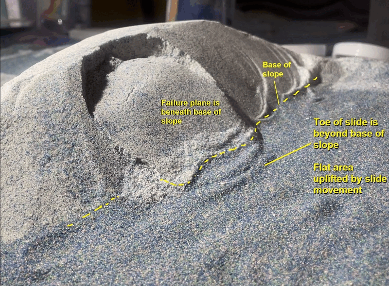
I drafted a basic cross section onto the image below. The red lines indicate the failure surface, which passes from the strong material down into the weak material to reach beyond the base of the slope.
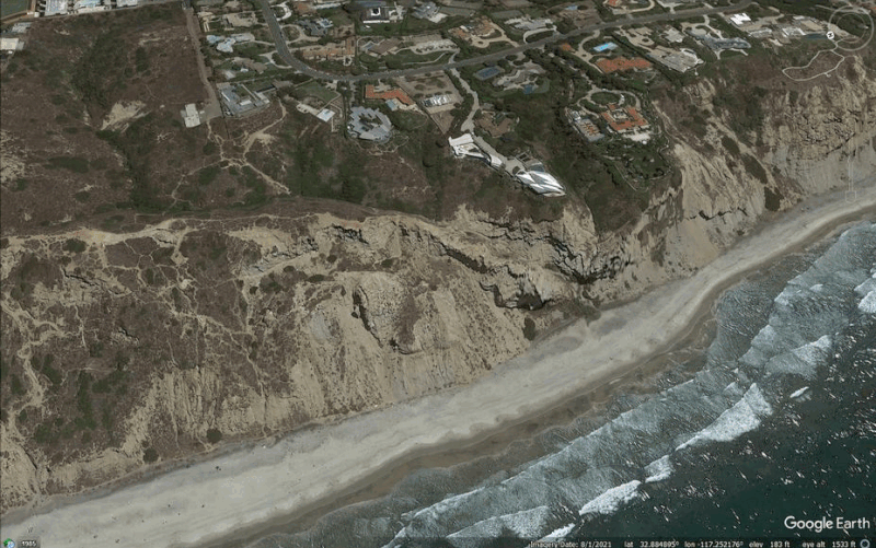
Looking at the real Blacks Beach slide from above, the same overall pattern is present. Notably, beach uplift occurred in a fairly small area. This may be a result of greater displacement of the slide block in this area, or failure may have occurred at the toe of the slope in other areas and remained above the deeper mudstones. The image was sourced from this video.
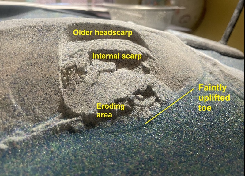
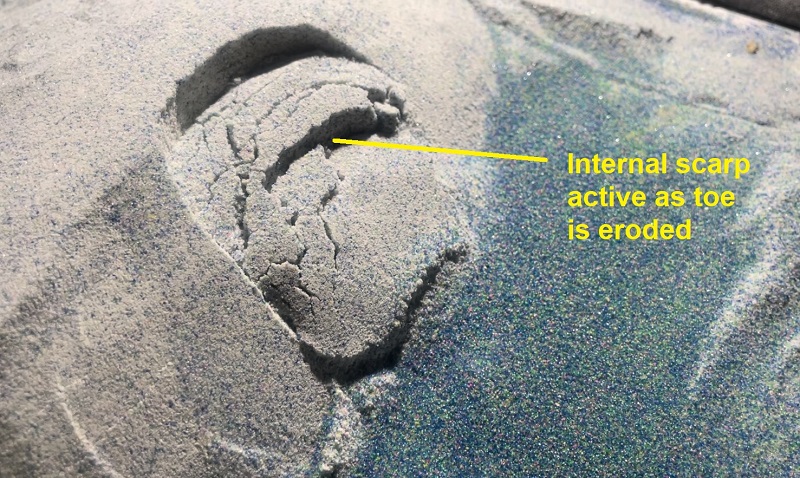
The Blacks Beach area has a history of slope failures (there was a big one here in 1982), and the January 2023 event certainly won’t be the last movement at this location. Erosion of the lower part of the slide by ocean waves continually destabilizes the slope, leading to more movement. The model shown in the GIF below demonstrates this process and is essentially a more “evolved” version of the previous GIF. I scraped away the lower part of the slide after initial movement, which led to development of a new failure surface within the initial slide mass. The lower slide block moves first, uplifting the dark sand beyond the base of the slope. The upper slide block then moves slightly. This sort of irregular movement can occur in reactivated slides as they shift and adjust to try to reestablish equilibrium between material strengths and gravitational force. As with the previous GIF, compression and uplift of the dark sand beyond the slope base occurs in conjunction with the downward movement of the upper part of the slide.
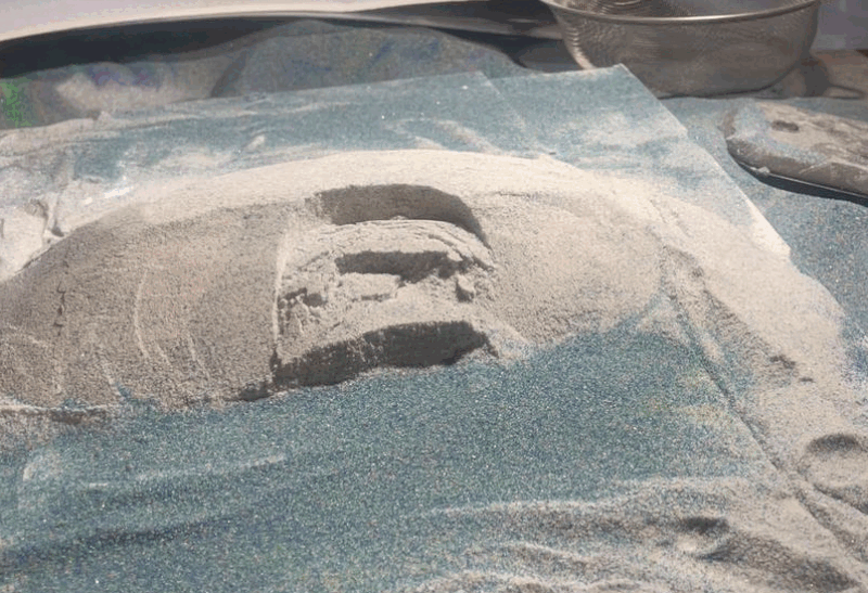
The respective scarps, the eroded portion near the base of the slide, and the uplifted toe are labeled in the image below.
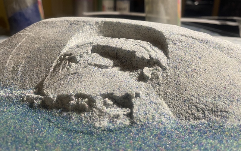
I think the additional images below just look cool. The slope in this model was made of “strengthened” sand, which fractured and broke apart nicely to replicate surface rock mass behavior.
Erosion undoubtedly plays a major role in past, present, and future activity of the Blacks Beach slide. Development of the uplifted toe provides a “counterweight,” so to speak, to resist additional slide movement. Erosional removal of the toe eliminates this resisting force and sets the stage for more movement. Kent Ameneyro did a great job of documenting the slide about a week after its occurrence, capturing great video of the eroded remnant of the uplifted area. The image below is a screen shot from his video, with a dashed line projection of the eroded material. The upturned layers that were within the toe are clearly visible.
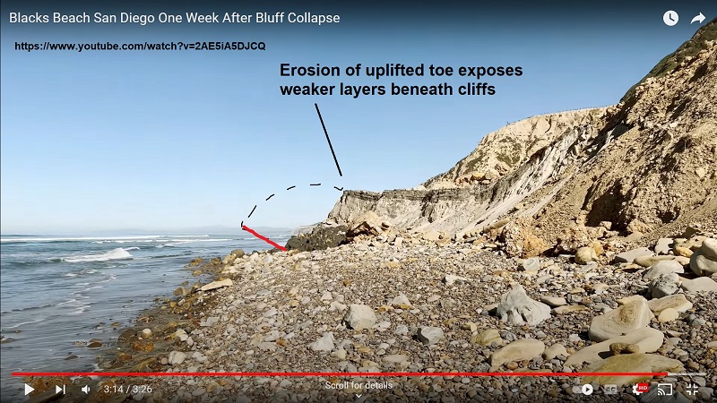
The screenshot below from this video shows a zoomed-out view. Considerable erosion of the entirety of the slide toe (not just the uplifted beach portion) can be seen.
Like many large-scale landslides with intermittent movement, the Blacks Beach slide area (the overall “slump complex”) is clearly visible in lidar-derived imagery. The GIF below fades a lidar overlay in and out to allow comparison of aerial topography to lidar imagery. The January 2023 movement is not shown here, but I attempted to outline the area that moved with solid yellow lines. The dashed line shows the older, uppermost headscarp. The uplifted toe is generally sketched in black.
Seeing a base failure landslide like this one professionally recorded first hand, and at close range, is truly remarkable. All of the videos of this failure, even those taken after, provide great information about how the slide developed and continues to evolve. Due to its size and location, stabilization certainly isn’t feasible, so all folks can do is sit back and wait for the next episode of movement!
-
Sandbox model anticlines formed above normal faults during extension
by Philip S. Prince
Reproducing fold structures observed in sedimentary rocks has kept geologists busy since the 19th century. Early model faults and associated folds (H. Caddell and B. Willis, for example) were produced by compressional deformation of a variety of layered materials, and an intuitive association certainly exists between buckle folding and squeezing/shortening a sequence of layers. Extensional deformation, however, can also produce folding if the dips of normal faults change with depth. I recently made the extensional anticlines shown below (white arrows) while trying out some new sand combinations. I thought they were quite nice…
These folds are “forced folds,” meaning that they are effectively collapse structures that develop as a moving mass of material deforms to match the shape of an underlying fault surface. The GIF below demonstrates this idea. Moving downward through the section, a steep-shallow-steep fault will produce a syncline-anticline pair, just like what formed in the models.
The same strong-weak-strong layer combination creates steep, then shallowing, then steepening fault segments in the models. Visibly different fault dips are quite apparent on the left sides of the model sections in the first image; the detail image below labels different strength zones.
Frequently, extensional anticlines are quite fractured and faulted, particularly along their crests. The models shown above retained generally continuous beds through the entire anticline due to the moderate strength of the green/blue and pink/blue layers. The sand in these layers is slightly weaker (less frictional) than the underlying yellow sand layers, allowing deformation to occur without creating discrete fault surfaces. The layers on the crest of the anticline are certainly stretched and thinned; they just didn’t accommodate the stretching and thinning through localized faulting. The left-dipping faults above the anticlinal crests (yellow arrows, below) are an expression of the stretching above the fold crests; this stretching occurred above a shallowly-dipping segment of the deeper fault.
The white arrow in the image above (upper model) points out another purely extensional anticline that develops due to abrupt steepening of a normal fault at depth. Folds like this are quite interesting, and they do actually result from localized reverse faulting and “passive” compression in the hanging wall. I have modeled this process before, as well. Like the models shown here, mechanically different sands are necessary to create the passive compression.
The model shown below might have developed folding similar to previous examples with more extension. The dashed black line and question mark suggest a possible location for the next fault to develop. If faulting occurred in this position, a narrow, almost “pointed” anticlinal structure might have developed. The dashed line position is, however, very close to the main breakaway fault at the right side of the graben, so it might not be a reasonable place to expect the next shear plane to develop. Ultimately, this model is mechanically different from previous examples (stronger gray basement, thicker brittle yellow section), so different fault spacing and patterns are expected.
Like all sandbox models–and real geologic structures–materials present in the layer packs shown here dictate the geometries of the folds and faults that form. Perhaps the most interesting aspect of this entire post is the similarity between the first two models shown. They are structurally quite similar, but they weren’t made it the same model run…
The model with green-and-blue basin fill was made about 1 week after the model with pink-and-blue basin fill. The models used the same combination of essentially mechanically identical materials and were extended the same amount, so the final model geometries were generally the same, despite being produced in two different modeling sessions. This reproducibility is a nice expression of the fundamental frictional relationships that govern Mohr-Coulomb failure at all scales.
-
Erosion and scour in sandbox model debris flows (microbeads and cohesive substrate)
by Philip S. Prince
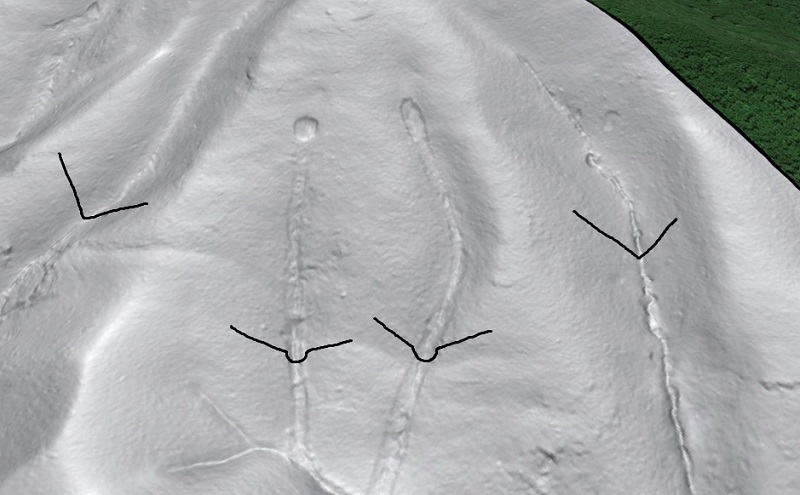
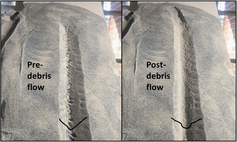
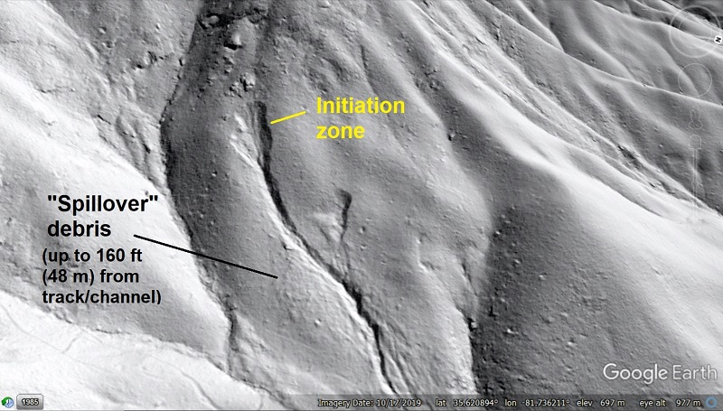
The speed and mobility of debris flows make them particularly dangerous among landslides. Debris flows move so quickly because they are fluidized masses of saturated soil, boulders and rock fragments, wood, and water, which causes them to erode or scour their flow path and accumulate more material than initially failed on the slope. The eroded track left by the scouring process is often clearly visible in lidar imagery, as in the case of the two debris flows shown below. These flows occurred in July 1995 near Buena Vista, Virginia, in the Appalachian blue Ridge. The respectively round and elliptical failed areas, along with the scoured tracks, stand out in comparison to “normal” ravines and channels on the slope.
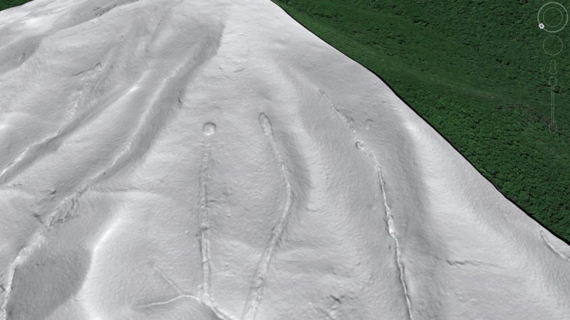
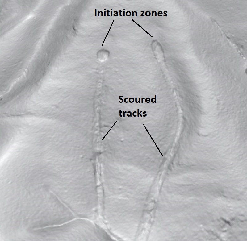
The failure scars (at the head of the scoured tracks) are about 65 ft (20 m) wide. The flows were about 25 years old when this Google Earth imagery was taken, and forest recovery in the scoured tracks is still limited to hardy species like pines. Looking more closely at the scoured tracks, they show a U-shaped profile compared to the typical V-shaped profile of channels or ravines sculpted by water alone.
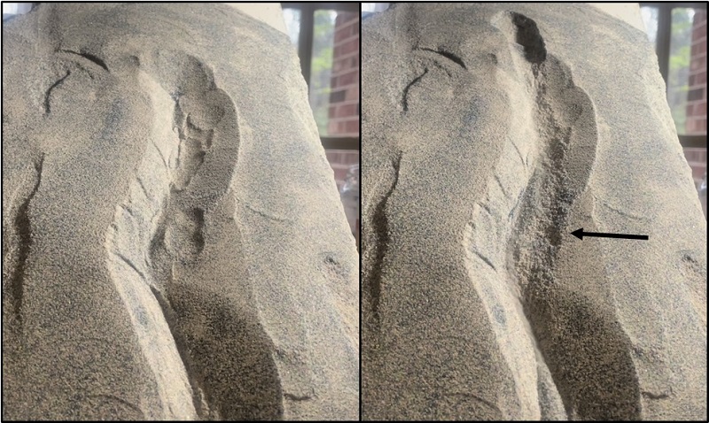
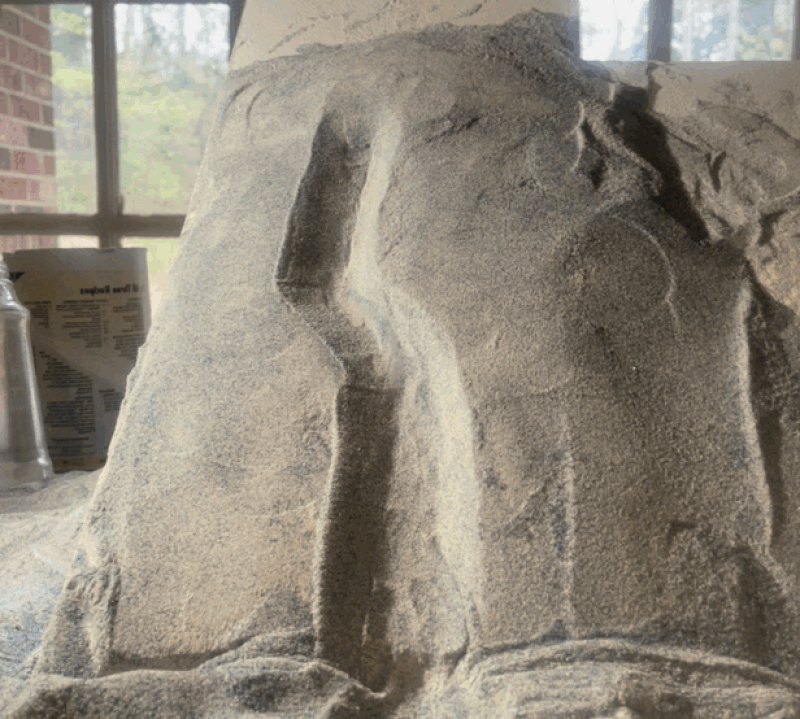
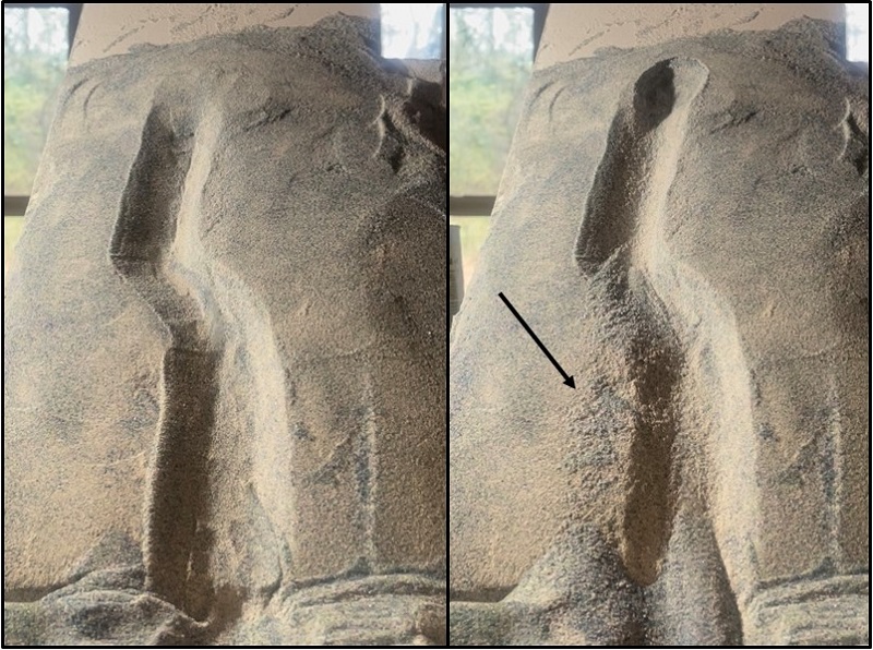
I look at these scoured tracks in lidar imagery all the time, and I wondered if might be possible to use granular analog materials to create similar eroded tracks in a sand model. Using a sand-flour mixture to make a cohesive slope was a V-shaped channel sculpted into it, I triggered slides of glass microbeads at the channel heads. The microbeads tend to fluidize when they are moving and colliding with one another, producing a dry analog for a natural saturated flow with lots of rocky debris. As seen below, the model flow does indeed erode the underlying slope and entrain the eroded material, added to the flow volume. I roughened the bottom of the initial channel to make the results of the scouring more noticeable.
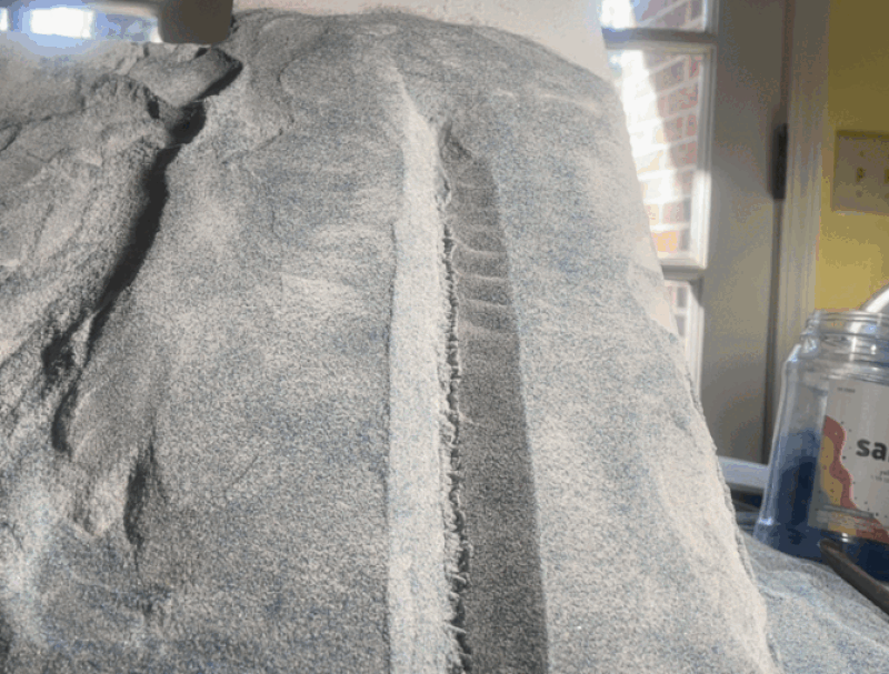
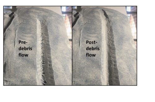
This is a simple model, but the effects of the flow on the initial slope condition are easy to see. Greater flow/track length would be good, but keeping the cohesive slope material stable on top of the tilting model base is difficult, and only gets more difficult as the model is scaled up. The flow is the most erosive towards the lower part of the model channel, where it is most concentrated. The image below provides a nice start-to-finish comparison.
Debris flows also surge up slope due to their momentum as they move around channel bends. Evidence of this process is visible in lidar imagery, as in the case of the 1995 debris flow shown below, which occurred near Graves Mill, Virginia. Like the previous example, vegetation is yet to fully recover. The transparent red outline shows the limit of scouring by the flow; the thin blue line shows the present-day water channel. Arrows show where momentum of the flow caused to it to run up, or superelevate, on the slopes.
The same model flow setup will produce some amount of the superelevation effect, along with scouring, if a curving initial channel is constructed. The GIF below shows one experiment.
The model flow superelevated twice, with the most obvious scour indicated by the black arrow. Removal of the surface lumps and bumps from the starting channel (left) is apparent in the post-flow appearance (right).
Another Graves Mill lidar example is shown below, with arrows indicating subtle evidence of scour due to superelevation of the flow. More on this event and its lidar signature can be found at this link.
Another curving channel example is seen below. This one also superelevated twice, with the second superelevation leading right into the zone of deposition. These flows don’t go very far once they leave the steep portion of the slope/channel because they are dry…see the video link at the end.
Comparing pre- and post-flow imagery shows erosion by the flow clearly, with initial texture in the channel scoured away where the flow was most concentrated.
A final example of flow behavior from McDowell County, North Carolina, shows how flow material can completely overwhelm a shallow channel due to volume or velocity and spread out over a flat slope. The transparent red area shows surfaces affected by the flow; whether the textured area to the right of the channel is eroded or holds deposited material (or both) is not entirely clear.
The following GIF shows this type of movement, with “spillover” debris leaving surface texture outside of the pre-formed channel.
Situations like this are actually quite common in the southern Appalachians, particularly with flows that occurred during the most extreme precipitation events (more than 10 in/25 cm of rain in less than 10 hours). Storms that generate this much rainfall have produced several “splashy” flows in which rock and boulder debris has surged out of channels and cascaded across generally planar slopes, often for significant distance. The lidar signature of this type of movement can be subtle, but it is identifiable once you’ve seen it. My main purpose in making models like these is to support pattern recognition in remote sensing, and this model came out very nicely.
These out-of-channel surges are not dramatic in lidar, but they do promote thought about debris flow mobility and just what parts of steep slopes are actually safe during extreme rain events.
The following video link shows footage of all of the models, along with the deposits left by the models. Because they contain no fluid, the flows grind to a halt fairly quickly when slope and velocity decline. Most deposits end up preserving a “jet” of microbeads within a broader area of less mobile material, including what the flows scour from the channels. In real, saturated flows, the jets of microbeads would be actual fluid material, which would blast through the deposit to leave a channel flanked by levees of coarse debris.
You May Also Like
Pleistocene Coastal Plain sand dunes and the value of pattern recognition in LiDAR interpretation
Lidar reveals geologic details of the “worst” coal mine in the Valley of Virginia
Lidar highlights impressive landslide density on the southern Appalachian Blue Ridge Escarpment, western North Carolina
-
Negative inversion of a sandbox model thrust fault
by Philip S. Prince
Inversion of normal faults during compression is a popular topic in structural geology, but thrust or reverse faults can also be inverted by extension. Like inverting normal faults, favorable fault dips are an important part of this process, particularly when it is reproduced in a sandbox model like the one shown below.
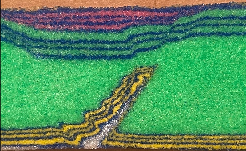
This model developed an initial steep thrust fault due to oblique shortening. The thrust, along which the yellow layer moved up-section, reactivated during direct extension to offset the interebedded green-blue and pink-blue horizons. These interbedded horizons post-date compression and pre-date extension. The annotated image below shows the main thrust fault beneath the displaced yellow interval and the associated extensional fault segments. The yellow fault segment was the first to move during initial extension; the black extension of the main thrust plane began moving later during the extensional phase. The white arrow indicates a purely extensional segment that expanded off of the existing thrust during reactivation…the layers it offsets were yet to be deposited during the compression/thrust phase.
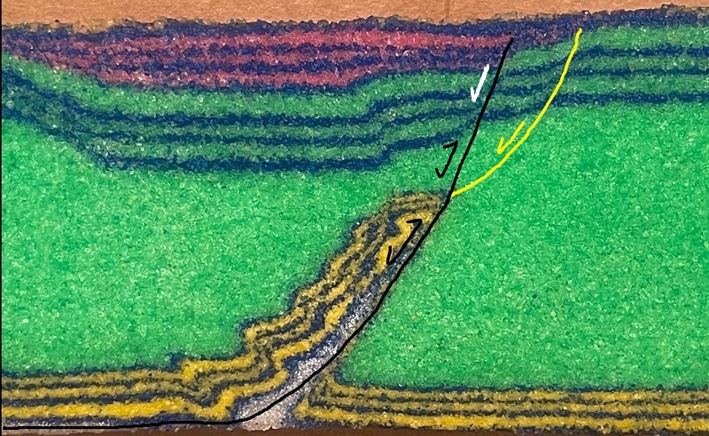
A particularly interesting detail of this model is the apparent reverse fault and gentle anticline in the blue-green section above the yellow thrust structure. Though it initially appears related to the thrust/compressional phase of the model, it is actually a purely extensional structure related to downward steepening of the initial extensional fault movement. The image below highlights the fault segments moving during initial extension; the abrupt downward steepening as the shallow fault deflects into the thrust plane forces the folding in the blue-green sequence.
Development of this model centers around the steepness of the initial compressional/thrust structure, which is steep because of the strongly oblique shortening that produced it. Direct shortening would have produced a shallower fault which would not reactivate during extension. The GIF below gives an overall sense of the orientation of oblique shortening, followed by direct extension.

During the extensional phase, faint evidence of the various extensional fault strands and the associated folding can be seen on the surface of the model. In the images below, locations of these features are indicated on the cross section slice of the model already shown.
The deformation sequence of this model involved considerable syn-compressional deposition, with green sand deposited along the flanks of the growing thrust anticline. This setup was used to produce the final compressional geometry with the yellow interval on the thrust hanging wall, completely surrounded by green. The yellow sand (dolomite sand) is stronger and more brittle than the green sand (quartz sand), so this geometry produces an interesting strength contrast zone within the layer pack. Drawing faults and the location of the pre-shortening surface on the cross section would look something like the annotated image below.
This model is effectively the inverse of a normal fault reactivation or basin inversion setup, which would require direct extensional motion followed by oblique shortening to invert the existing normal faults. At least in the sandbox model world, both of these inversion approaches require oblique compression to produce thrust or reverse faults of sufficient steepness to match up with normal faults, whose dips are always steep in these models. A basin inversion model produced by the “inverse” of the setup shown here is seen below.
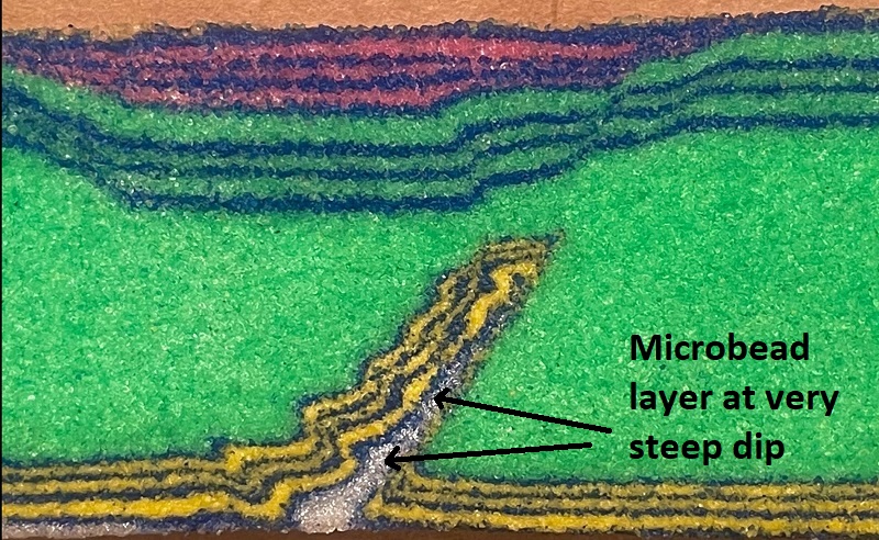
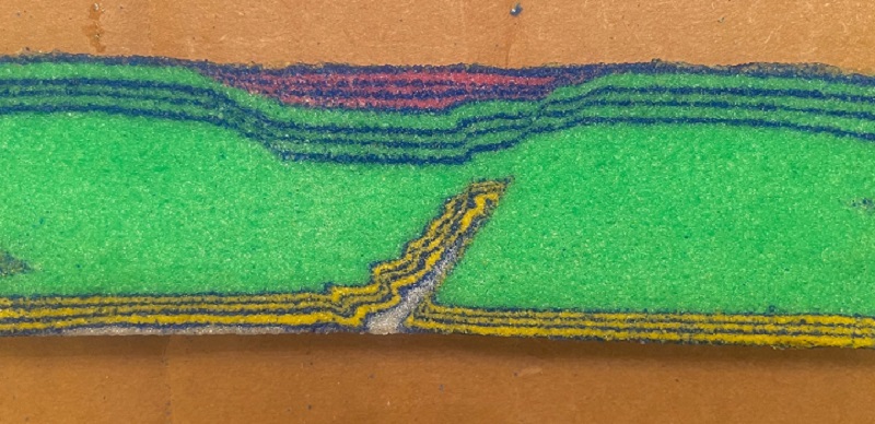
A detail of the thrust inversion setup that may impact the slightly lower dip of the initial normal fault segment is the presence of the weak microbead decollement layer on the thrust ramp. During shortening, the microbead layer is carried up the ramp. The microbeads have very low internal friction and are exceedingly unstable on the ramp at its high dip. As soon as compression is released and the layer pack can “relax,” collapse within the steeply dipping microbead horizon begins immediately.
Finally, the overall appearance of the model slice is shown here. This setup consumes a regrettable amount of whatever color of sand is used for the growth sequence. The model was developed on a planar, flat base plate. The faint curve at the base seen here is the result of careless slicing and drying!
While this is a very idealized setup with a specific outcome in mind, structures like this do develop in settings where stress regimes can change significantly and the potential for rapid subsidence and syn-deformation deposition is high. Back-arc settings are a good example, as subduction angle, behavior of the sinking slab, shifts in orientation of plate motion, etc. can greatly alter deformational and depositional conditions in the overriding plate. Such a setting might experience extension and deposition, localize compressional inversion to produce isolated thrust structures like the one shown above, followed by a return to extensional or transtensional stress regime to cause collapse. I like this model because it nicely demonstrates the importance of stress field orientation and the independent variable of material strength on deformation patterns.
You May Also Like
Real sandbox model meets “numerical sandbox” model…an interesting comparison of dry granular media and discrete element simulation
Erosion and scour in sandbox model debris flows (microbeads and cohesive substrate)

The Blacks Beach landslide: Why did part of the beach rise as the cliffside slid down?
-
Making lateral spread landslide models with glass microbeads…and lots of shaking!
by Philip S. Prince
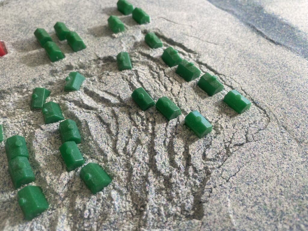
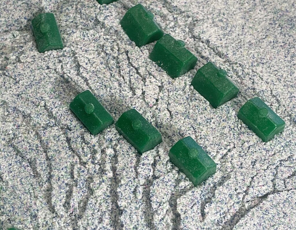
Many aspects of geology are fundamentally related to material movement, but geologists can often only examine the final results of the movement for reasons of physical scale, time, and safety of personnel. Earthquake-related lateral spread landslides are a good example–they create incredibly dramatic landscape damage, but filming one from an appropriate vantage point during intense shaking is nearly impossible. Physically modeling lateral spreads is also problematic because of the soil liquefaction involved; it’s tough to combine dry and wet granular media and keep them (and their properties) separate. An illustrative, and entirely dry, lateral spread model can be made using glass microbeads beneath a cohesive sandpack, which I make by combining sand and flour. During shaking, the microbeads behave like a viscous fluid and deform the overlying sandpack. The images below show one such model I recently made. I decorated the pre-slide landscape with Monopoly houses and hotels, which got caught up in the action.
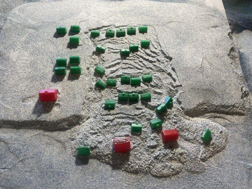
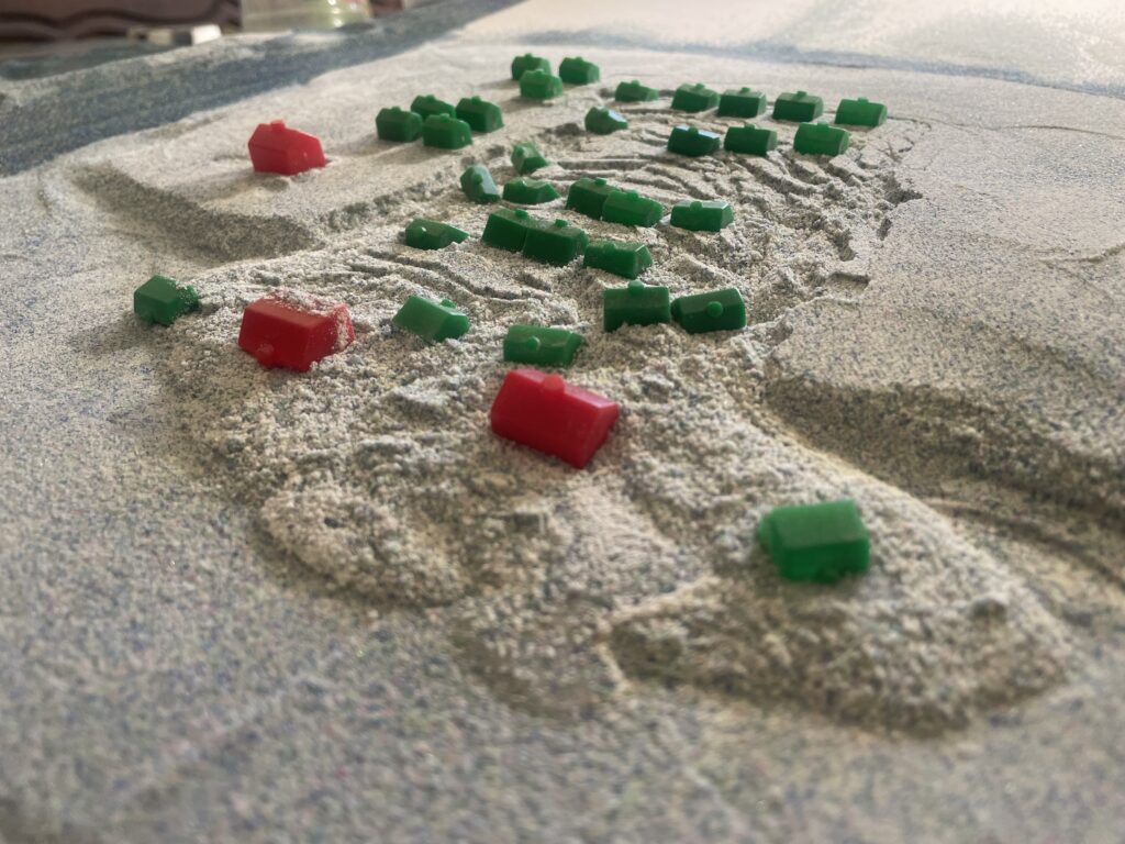
Lateral spread models made in this way are entirely conceptual and illustrative, but they look cool and do reproduce details of ground deformation above a seismically liquefying horizon. A sandpack is constructed over a layer of glass microbeads, and the whole baseplate under the model is shaken to cause the microbeads to “liquefy.” Deformation to the cohesive sandpack above the microbeads is visually interesting, with complex arrays of scarps and rotated blocks, as seen below.
No effort is made to scale the shaking; the model is simply shaken until the microbeads lose strength, presumably due to reduced sliding friction against one another during acceleartion. The in-motion appearance of these model is fun to watch, and is the main thing to take away from this post. The video linked below shows the model above, along with two others. The video shows shaking and failure at 1/2 speed, which is a bit easier to watch.
While the frequency and amplitude of shaking are exaggerated to get the desired outcome, the lateral spreads made using microbeads display some realistic details that are useful for students or non-geologists to see and connect to a formative process. Block rotation and tilted or sinking of structures within the spread is one such detail, as seen below.
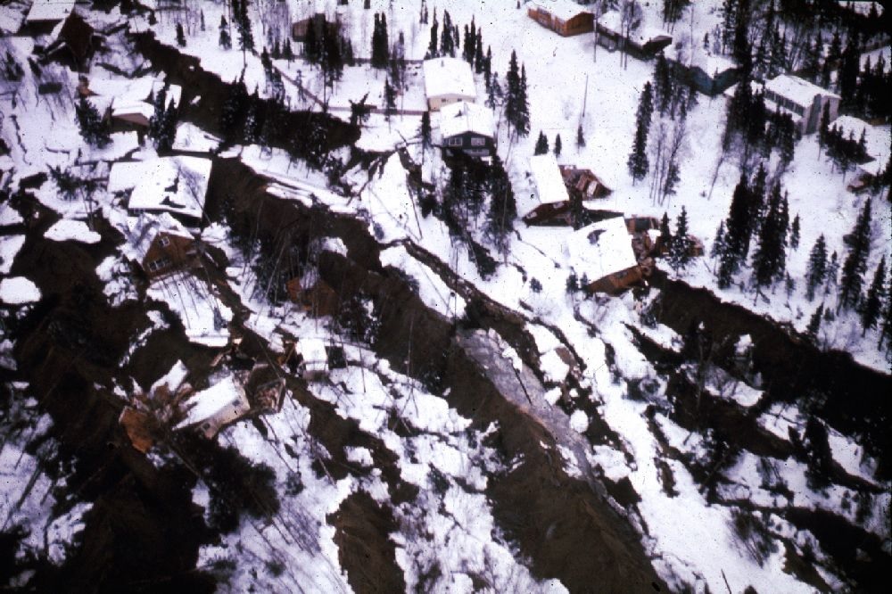
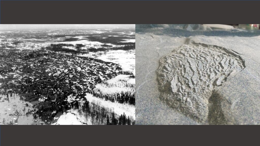
I tried to make these match some of the Turnagain neighborhood images from the 1964 Alaska quake, with acceptable result. The image below is from The Atlantic, I believe.
The model lateral spreads also move with gravity and require very, very little slope to do so. Tilting the baseplate only a few degrees will lead to downslope flow. The models shown above used a slightly (3 degrees?) tilted setup and a daylighted microbeads layer (the model starts with a “bluff” below the houses) to create a strongly directional spread. The overall appearance, along with the finer details, can be made to match photographs of real lateral spreads very closely.
Lateral spreads affecting infrastructure can also be modeled. The experiments shown below induced lateral spreading below a model embankment. Again, with slight tilt or asymmetry, the spread that develops is directional. The arcuate scarps in the model spreads below turned out well.
These models confined the microbeads in all directions, and they “sloshed” significanlty from side to side; this movement is easily visible in the video linked below.
The final geometry of these spreads was remarkably flat, with a gently raised toe bulge and equally low slope slide head. Head and toe reaches this equilibrium geometry when the microbeads layer was at its weakest.
Inducing a lateral spread beneath a symmetrical embankment-type structure with no tilt produced a variety of results, but bi-directional spreading and toe compression are possible. Sloshing was a problem here, too–see the previous video link. Shaking in a single direction meant that the final outcome related to orientation of the embankment to the shaking direction.
I wanted these models to compare with one of the more widely distributed examples from the 2018 Alaska earthquake, where a road (Vine Road, I believe) experienced a bi-directional spread with two compressional toes. The image below is from the USGS My setup needs more work, but the potential is there…
The obvious drawbacks to these models are the lack of true pore water-induced liquefaction and the exaggerated shaking and sloshing, but these models are easy to set up, easy to break down, and make the connection between shaking, distinct material behaviors, and earthquake/slide-related landforms easy to appreciate. Vibrating the base plate might also produce a good result, but I have not constructed a rig to produce it. If anyone gives it a shot, let me know!
-
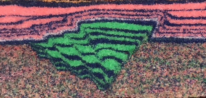
What’s under that anticline? Fold-thrust belt interpretation ideas from geologic sandbox models
by Philip S. Prince
A look around this website will make it pretty clear that I like sandbox models, mostly because I think they look cool. Beyond aesthetics, geologic sandbox models can be useful tools for thinking about approaches to geologic interpretation and learning to visualize and reproduce realistic structural styles. The model shown below illustrates an interesting case of how surface geologic mapping, remote sensing, and an understanding of how various sedimentary rock types respond to tectonic deformation could be used to figure out what sort of rock structures might be present under a given point on the land surface. Like many of my models, this model represents a sedimentary fold-thrust belt whose thickness would be measured in terms of miles or kilometers. Specifically, the model is intended to reflect a “young” thrust belt which has not been significantly eroded since the end of the crustal shortening that formed it.
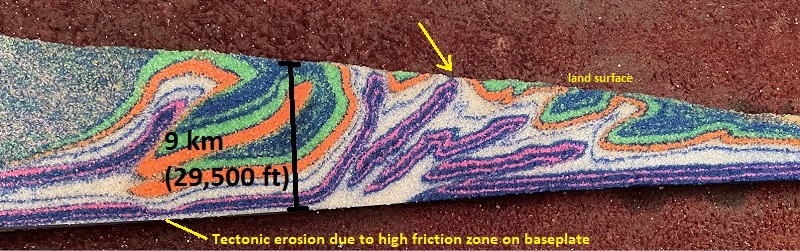
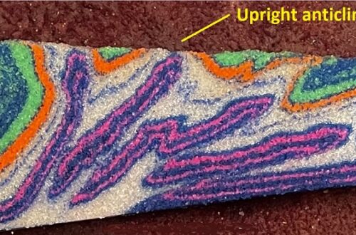
This model definitely satisfied the “looks cool” requirement, but it also contains a particularly interesting structural feature: an upright anticline exposed at the model’s surface, which is indicated by the yellow arrow above. This surface fold is interesting because of what is underneath it, namely several “slices” of the pink/blue interval stacked on top of each other. Complex structures like this are common in Earth’s sedimentary fold-thrust belts and are tough to fully interpret without seismic surveys or drilling through them, but field- and concept-based information can be gathered to at least give some idea of what might be beneath an anticline like this one. I offer up a few of my own thoughts here, and there are undoubtedly many other possible strategies.
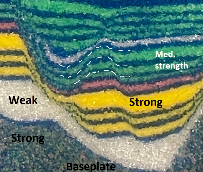
First, the anticline itself is worth a closer look:
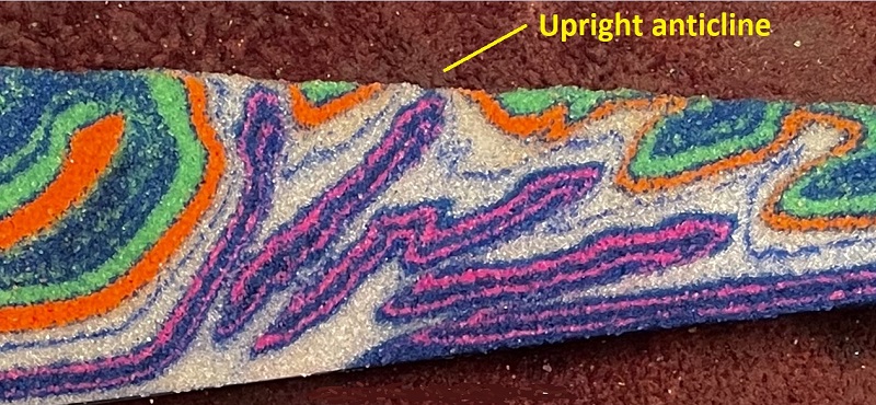
The anticline is upright, and the orange and green layers that define its limbs have comparable dips. Dip steepens significantly towards the core of the anticline, with layers at the right hand edge of the pink/blue interval being nearly vertical next to the much shallower orange layer. The white material (glass microbeads) is much weaker than any of the colored sand layers; it represents shale in terms of real-world rock types. A geologist cruising across this anticline would certainly note the presence of the shale and how it separates shallower dips from steep dips.
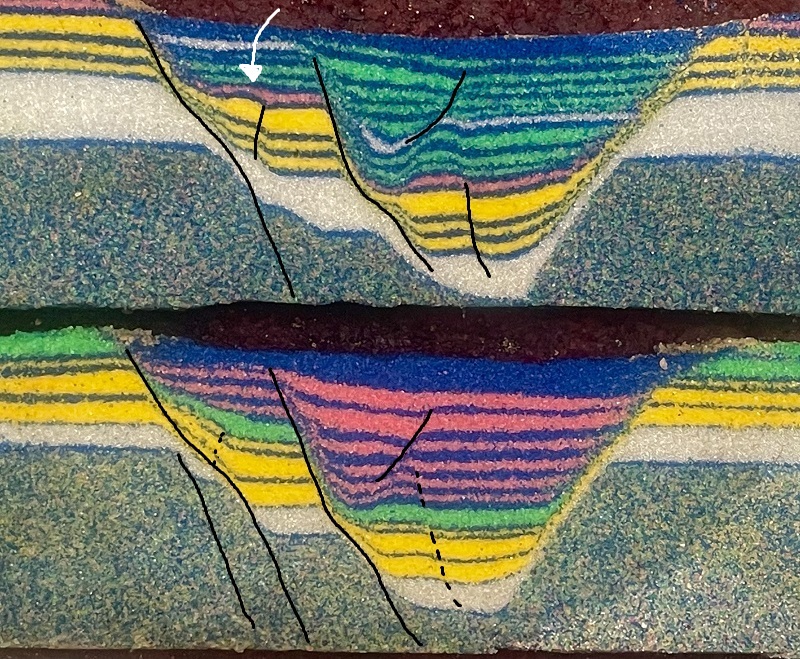
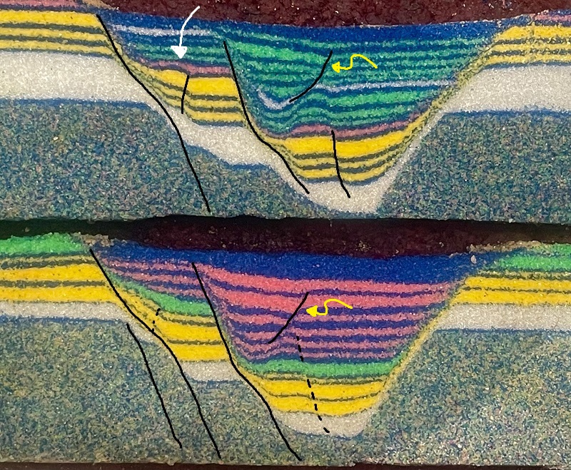
Moving left of the anticline, a geologist would encounter a thrust fault that has been tilted backwards until it is slightly overturned. This is strange, and will be significant later. The fault itself would be obvious due to the rock types it separates, but its orientation would be perplexing.
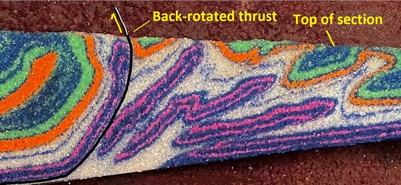
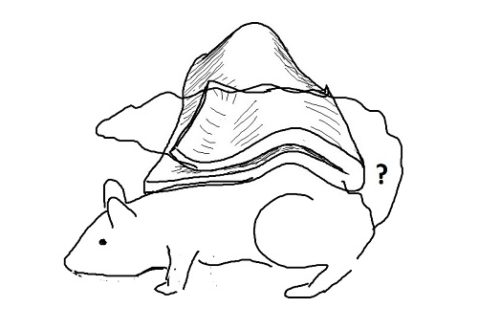
Moving to the right of the upright anticline, a geologist would encounter a thrust fault placing the orange and green layers atop a much younger blue layer that defines the top of the folded/thrusted section of layers (“top of section,” above). This is a notable feature, but it doesn’t help much with figuring out what is under the upright anticline, and might even cause confusion (more on this below, too). This potential confusion arises largely from the shape and width of the anticline, which indicate that it doesn’t extend terribly deep into the thrust belt, as diagrammed below.
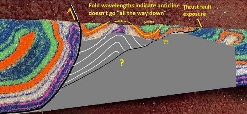
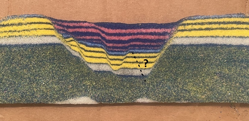
The width/wavelength of the anticline and its neighboring synclines are very good evidence that the upright anticline is likely developed above a thrust fault, represented by the black line above the question mark. This bit of information is a good starting point, but determining what layers are below the thrust fault is another challenge….and given the thickness of the fold-thrust belt implied by the big syncline on the left, whatever is down there is likely stacked on top itself a few times. The thrust fault to the right of the anticline, which places orange and green atop the younger “top of section” layers, might suggest orange and green extend beneath the upright anticline. This possible geometry is sketched below. Note reference to structural repetition and particularly dip in the deep syncline at left as an indicator of thrust belt thickness.
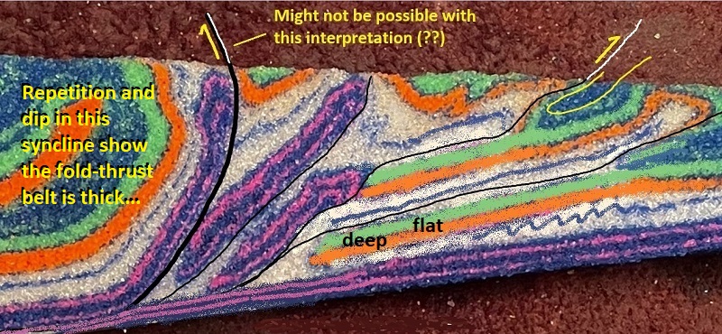
I sketched this up in an effort to offer an alternate subsurface interpretation, and I think it is “believable,” at least at a glance. It would be easily disproven, of course, by drilling or seismic data, but are there other, massively less expensive ways to tell that it is wrong? I think there are a few, starting with the back-rotated thrust fault. I don’t think the geometry sketched above would produce or preserve the back-rotation of the fault as it exists in the model. I think the additional stacking of the pink/blue interval (meaning more “slices” with thrust ramps) is necessary to produce the back-rotation, and the geometry drawn above would actually begin to “un-rotate” the back-rotated thrust if the deepest orange-green flat (“deep flat”) advanced further. I haven’t actually sketched all this out, but I am suspicious that it’s legitimate…
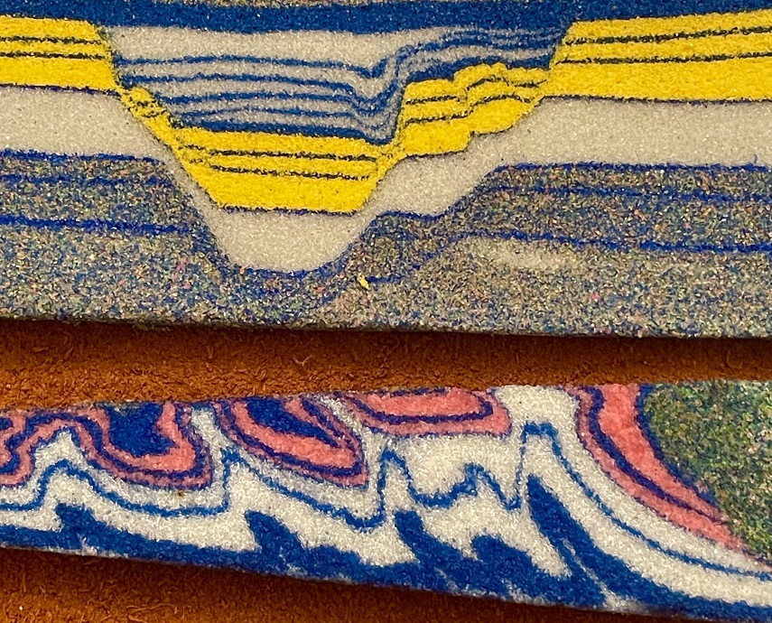
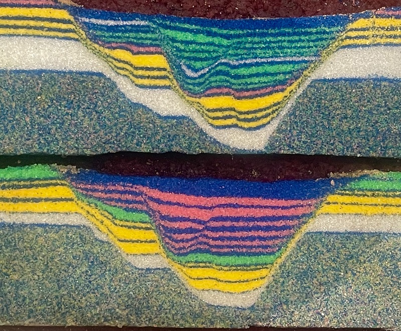
Another useful approach would be additional mapping in the vicinity of the upright anticline. Additional sections from the model are shown below, and one of them shows a tight fold instead of a thrust to the right of the upright anticline.
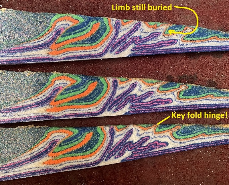
If enough of the forelimb of the fold could be seen to convince the geologist that the structure is not in the hanging wall of a thrust, at least one thickness of orange and green would be confirmed to not extend under the upright anticline. This detail would suggest fault repetition of pink/blue and direct the geologist towards a more accurate interpretation. Were the fold hinge labeled above not visible itself, seeing the upturned footwall limb of the same structure in a deeply eroded area would have the same useful effect of showing that the upper orange-and-green footwall does not extend under the upright anticline.

Beyond field mapping, examination of gravity anomalies in this portion of the fold belt would also be useful in suggesting what stratigraphic interval is repeated below the upright anticline. Nearly all of the fold-thrust belt’s thickness below the upright anticline is made up of the repeated pink/blue horizons. If pink/blue were a limestone/dolomite (carbonate) interval and orange/green were a sandstone-shale interval, a gravity high would occur in the vicinity of the anticline due to the stacking and concentration of the dense carbonate rock. If pink/blue was sandstone and orange/green was carbonate rock, a gravity low would occur beneath the anticline.
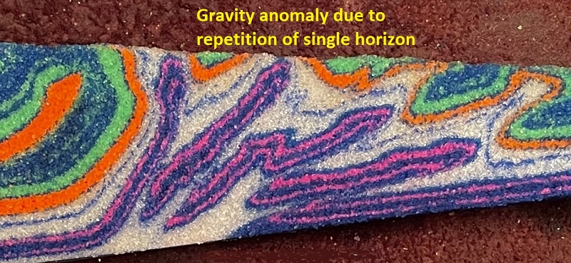
In either case, such a gravity anomaly would very quickly eliminate the repeated orange/green model sketched earlier in the post and confirm repetition of pink/blue. This approach has been used in the Appalachian Valley and Ridge, and I summarized it in a post a few years ago.
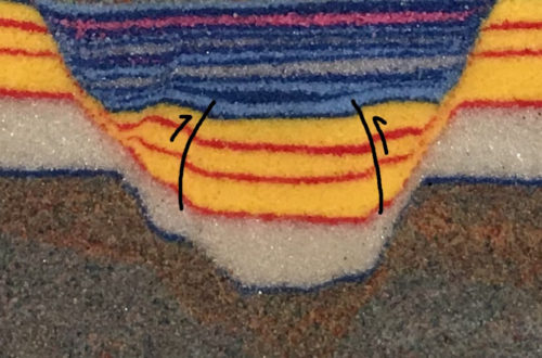
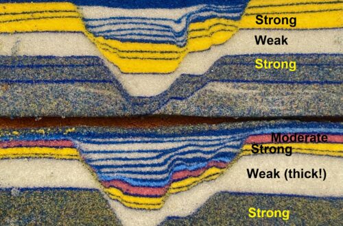
Even if repetition of pink/blue beneath the anticline was confirmed by field data and additional remote sensing like the gravity anomaly approach, details of the structure would still be very difficult to sort out. Thickening of the weak white “shale” layers is significant, with the middle shale layer (number 2) showing extreme thickening below the upright anticline.
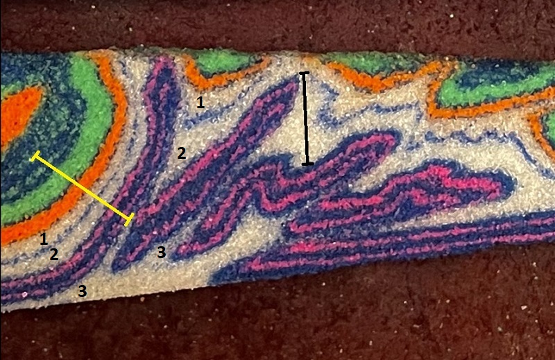
The yellow line above shows the thickness of the full section involved in folding and thrusting (much of it is, of course, eroded away above the upright anticline). The black line shows thickness of shale 2 beneath the anticline, which is (depending on where it’s measured) over 75% of the full section thickness. The thickness reflects shale 2 being “scraped off” a lengthy portion of pink/blue and piled up in one spot, but it still might seem odd to interpret such an extreme thickening. The thickening shown above is indeed localized, and inspection of the other sections in the earlier image shows variations on how the weak white layer moved around and thickened within the model.
I think that interpreting at least two repetitions of pink/blue beneath the upright anticline would be possible from surface and gravity data at the erosional level of the model. Going deeper without some information about the overall thickness of the fold-thrust belt would be tough, but an understanding of structural style in the area, such as the tendency of pink/blue to stack on itself, might be combined with overall surface geology and the big syncline at left to actually estimate the thickness of the fold-thrust belt. Application of structural style might even lead a geologist to conjecture about thrust sheet C (below), as shown below. Seismic data would, of course, fix most of the problems discussed thus far!
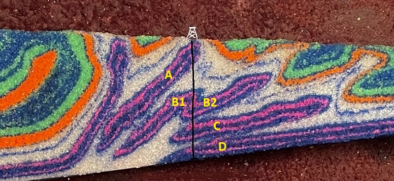
Drilling through the anticline to the base of the fold-thrust wedge would be the final word on just how many pink/blue slices are present, but even the well bore shown as a black line would pass through partial thicknesses on thrust ramps and require some thought. This well bore would then raise even more questions about how far to the right B2 and C extend, which really can’t be determined from surface data. Notably, both B2 and C have end in hanging wall anticlines that are directly below surface synclines.
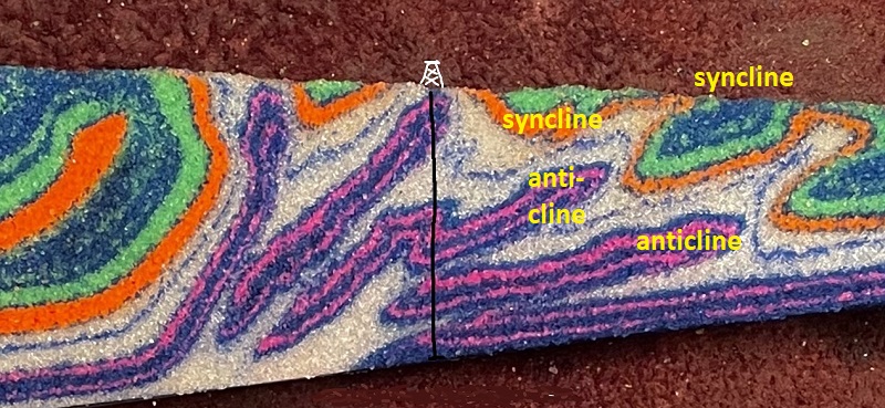
Anticline-under-syncline arrangements are actually reasonably common in shale-rich thrust belts where structures developed in stronger horizons (pink/blue or orange/green) shift slightly past each other within the weak shale layers. In reality, this entire post comes back to the presence of the “shales” (the white microbeads) in the model. The presence of the microbeads is fully responsible for the complex structural style seen in the model. A general conceptual understanding the way weak detachment layers impact thrust belt structure would be key to interpreting this system in the real world. Without consideration of how the weak layers control structure, figuring this system out-even with drilling-would be tough, to say the least!