-
Blowout landslides, part 2: Material movement, and did anything actually “blow out?”
by Philip S. Prince
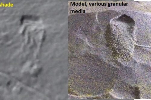
“Blowout” is certainly a peculiar name for a type of slide, but the lidar signature of blowout-type landslides legitimately gives the impression that a force from inside the hillside pushed material out. Observers of these failures developed the same impression, and even a basic physical model (below, right) of this failure style ends up looking like a big hole on a slope that soil spewed out of:
So, what actually happens when these slides occur? I have not personally witnessed one, but I think that a look at details of failure surface shape and the behavior of saturated soil during failure can be used to figure out why blowouts appear to “blow out” instead of just slide. In a second rare move for this page, I again link to an original post on the Appalachian Landslide Consultants site, which presents a host of sketches, a GIF of the model above, and a link to YouTube video of the actual New Zealand slide screenshotted below, which offers insight into the details of blowout material movement. The link can be found at the end of this post.
The most interesting part of this screenshot is the group of small trees being struck by fluidized slide material from the New Zealand failure–specifically the fact that they aren’t being knocked over!
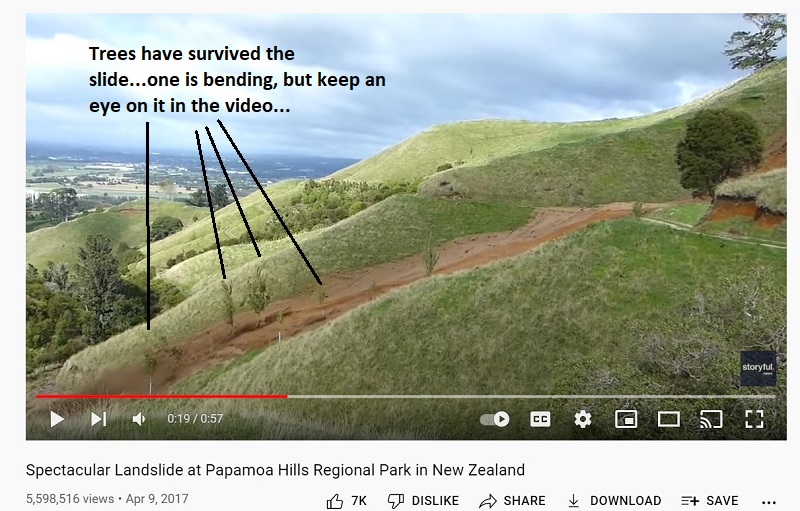
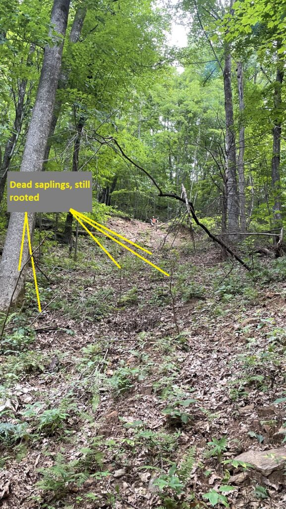
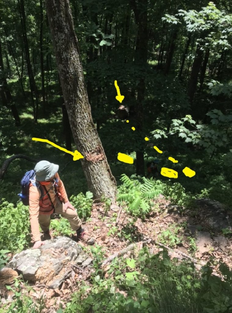
Lack of disturbance of the slopes below blowouts was remarked upon by both Eisenlohr (1952) and Hack and Goodlett (1960), with Hack and Goodlett going to the length of determining just how small of a sapling tree could survive a blowout strike in their study area. I have personally only seen one recent (1 year old) blowout in the field, but it presented the same intriguing lack of slope damage as observed by the earlier authors elsewhere in Appalachia. The photo below shows numerous small saplings killed by the blowout that were not uprooted or even flattened. Most of the tiny trees indicated below are less than 1/2 inch (1.27 cm) in diameter, and while they were damaged sufficiently to be killed, their modest root systems were clearly up to the challenge presented by the blowout material. Their root systems were not even exposed by physical removal of the uppermost soil horizon, which appeared essentially intact. The slide scar is visible in the background.
Preservation of small vegetation like this presumably results from extreme fluidization of the sliding–or more appropriately, flowing–mass, which moves like a slurry. Fluid or not, the slide material still contains large clasts, so the little trees presumably avoided these. The image below shows a detail of the colluvium involved in the failure, which exposes the bedrock colluvium contact. Some amount of fill was involved as well; just how much was unclear during this field visit.

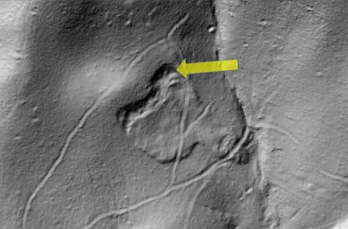
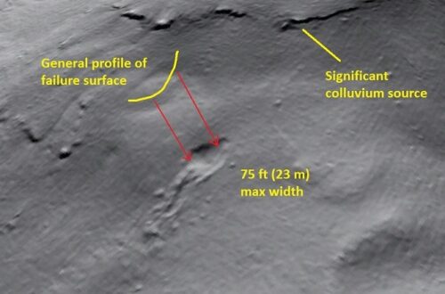
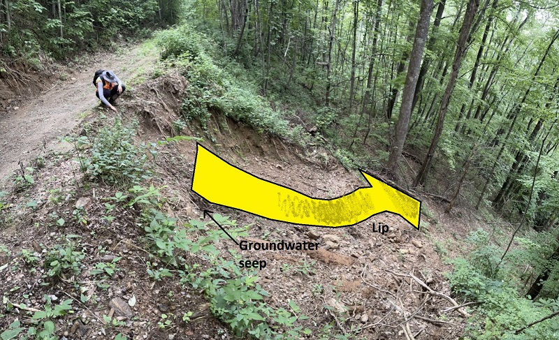
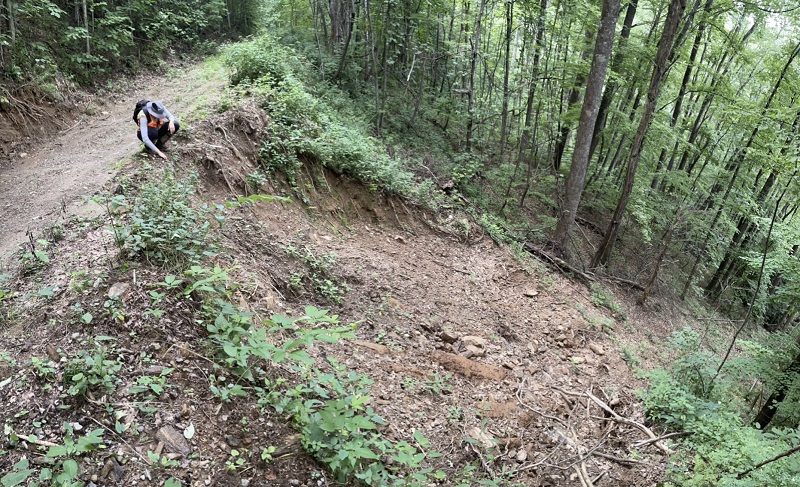
The scar left by this blowout also provides a look at the flat area that creates a lip at the base of blowout failure scars. Rapidly sliding, saturated material obviously moved up and over this lip without degrading it. This path would have caused the material from high in the failure scar to “ramp” out of the scar and fluidize, particularly if it accelerated quickly after initial failure. If observed from downslope, I’m sure this does indeed create the impression of material spewing out of the slope. The images below show the failure scar with and without annotation. Also notable is the seep/wet area, which persists here even in dry weather.
Considering this failure in comparison to the New Zealand failure is interesting, and I presume the degree of fluidization seen in the New Zealand failure likely occurred here to allow preservation of the sapling trunks downslope. Check it all out at the link below.
Link to second blowout post on Appalachian Landslide Consultants, PLLC page
-
Sandbox models with high-displacement thrust faults compared to features of some Canadian Rockies sections
by Philip S. Prince
Sandbox models don’t always produce the geometry the modeler wants, but with properly scaled materials, a “failed” model run can still produce worthy analog structures. I recently came up short on attempts to model some details of the southern Appalachian Valley and Ridge, instead producing structures reminiscent of some well-known Canadian Rockies sections. The Alberta section shown below was most recently (I think?) published in Mackay (2015), though I am unsure of its original origin (it can be viewed here without journal access). This section shows some interesting fault zone and thrust footwall details that unexpectedly popped up in my slightly-off-the-mark models. Note that the models don’t replicate the entirety of this section; they just reflect some of the structural styles characteristic of fold-thrust belts with high-displacement thrusts.
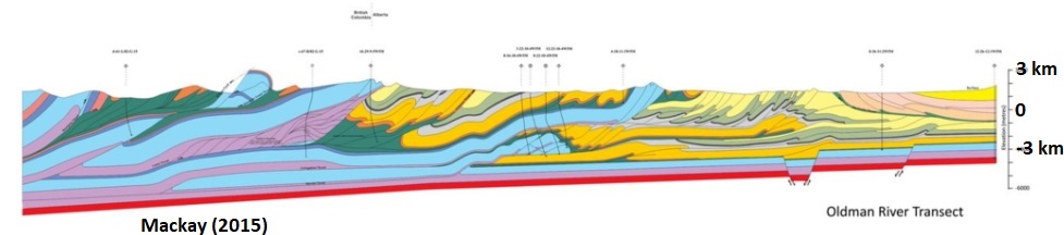

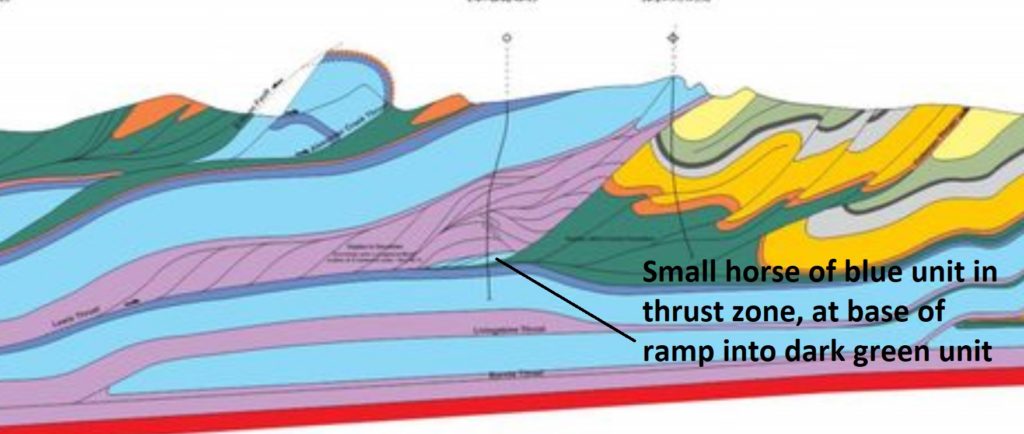
A favorite detail of this section is the thin “horse” block (an entirely fault-bounded piece of stratigraphy within a fault zone) being dragged along in the Lewis Thrust zone. If you look closely, you can see that the horse was penetrated by a well, which is presumably how its existence was confirmed. A zoomed look at the horse is shown below.
The model shown below contains a comparable small horse detached from the yellow layer in the footwall of the overlying large, high-displacement thrust sheet. This model horse consists entirely of the yellow bed and the thin, dark blue layer intended to highlight the yellow bed’s boundaries. Despite being folded on top of itself in a tight, overturned syncline, the horse is too thin to significantly arch the overlying thrust sheet, making its presence unnoticeable from the surface of the model.

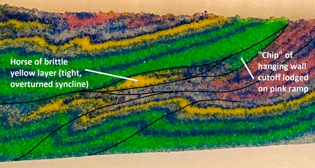
The thin yellow horse developed because the brittle yellow bed (dolomite sand; pink and green are quartz) is bounded above and below by glass microbead detachment layers. These weak bounding layers permit small sections of the single brittle yellow layer to be “torn off” of a footwall ramp and carried along within a thrust zone. Removal and transport of the horse occurred after the overlying thrust fault had already accumulated notable displacement–the horse is much closer to its own footwall cut-off than the leading edge of the green thrust sheet it to its footwall ramp. The position of the high-displacement thrust sheet’s ramp relative to the horse’s origin is apparent when the entire model wedge is shown.

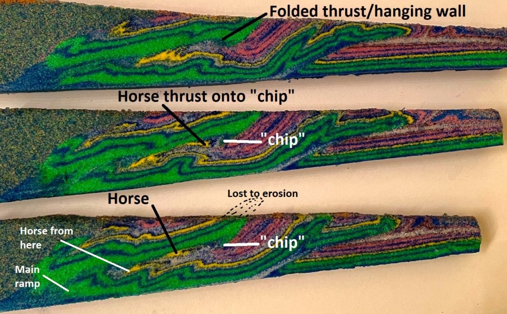
Other sections in this model showed a similar horse which had experienced more transport and lodged against the “chip” of green hanging wall strata stuck on the pink ramp. The model images below show this relationship–compare it to the previous horse images, where the horse has not yet reached the ramp zone.

This model section is interesting because the yellow horse is thrust onto older green layers of the “chip.” This relationship is possible because the green chip lodged early in the thrust sequence, with the yellow horse being detached, transported, and lodged later. I would be interested to know if relationships like this have been drilled through (or otherwise observed) in the Canadian Rockies section shown at the beginning of the post. The southern Appalachian Valley and Ridge hosts this type of geometry in several locations where numerous ramps and flat exists within the imbricated sedimentary section.
A second model produced a deep, sub-thrust ramp anticline similar to a feature beneath the Livingstone Thrust in the Canadian Rockies section.


While the model ramp anticline lacks the significant thrust displacement associated with the “real-life” structure, it produces no significant surface expression in the overlying thrust sheet, similar to the real anticline. Much like the small horse in the earlier example, the presence of the deep ramp anticline would not be immediately obvious from surface observation, particularly without some overall geometric constraints on the thrust belt’s architecture, such as its overall thickness. The presence of blind features like these beneath high-displacement thrust structures makes interpretation in thrust systems with many detachment horizons particularly challenging.
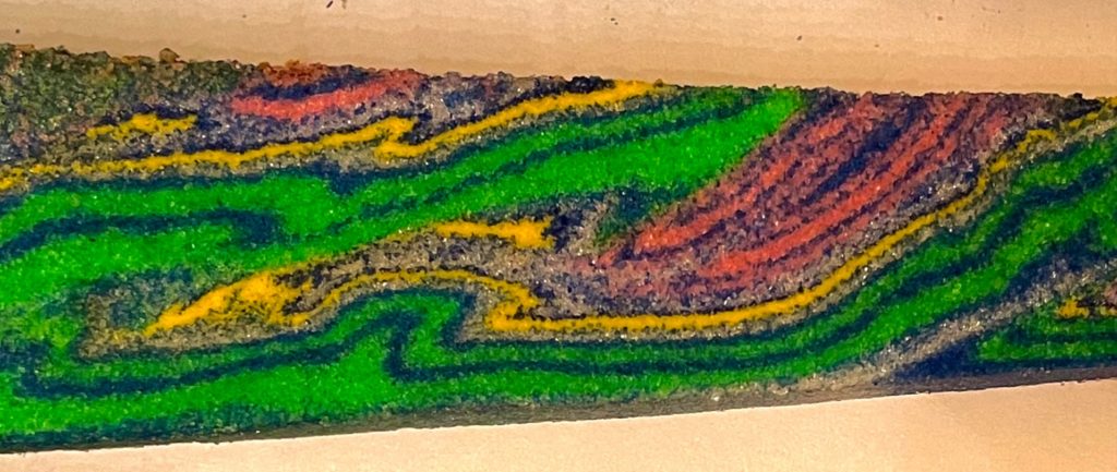
The “deep anticline” model also produced an interesting pair of anticlines near the hanging wall cutoff of the overlying, high-displacement thrust sheet. One anticline is associated with the cutoff of the deepest layer of the thrust sheet, while the second is developed by drag along the thrust.
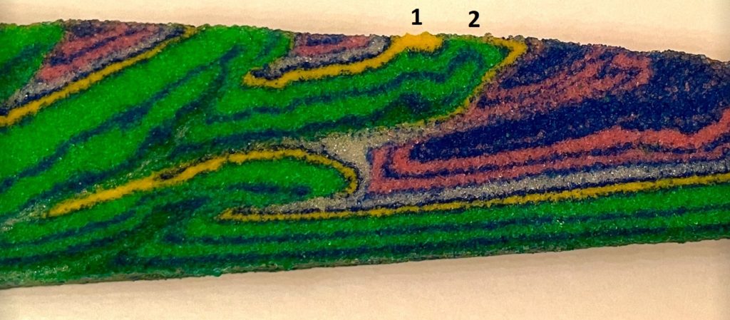
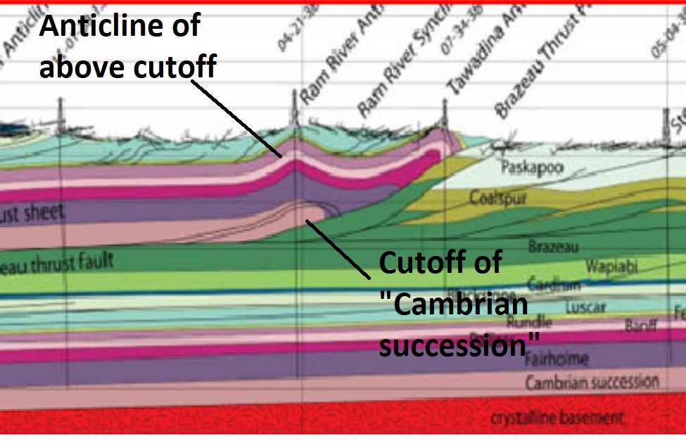
This geometry was reminiscent of the Ram River Anticline of the Brazeau Thrust system, shown below in a section sourced here.
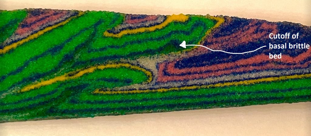
While the footwall of the Brazeau Thrust beneath the Ram River Anticline is generally intact and undeformed, the model’s thrust footwall hosts interesting upturned beds cut off by the thrust fault. Were the model a real thrust belt, drilling through the first anticline of the upper thrust sheet, through the thrust, and into the upturned footwall beds might be interesting, whether you’re into exploration or carbon storage. A hypothetical well is shown here…
…and after all of this, what was the intended, southern Appalachian-style model supposed to look like? Something like this, with a couple of thrust imbricates atop an undeformed flat footwall.

https://www.lyellcollection.org/doi/abs/10.1144/sp421.5
http://en.earth-science.net/en/article/doi/10.1007/s12583-017-0775-z
-
Real sandbox model meets “numerical sandbox” model…an interesting comparison of dry granular media and discrete element simulation
by Philip S. Prince
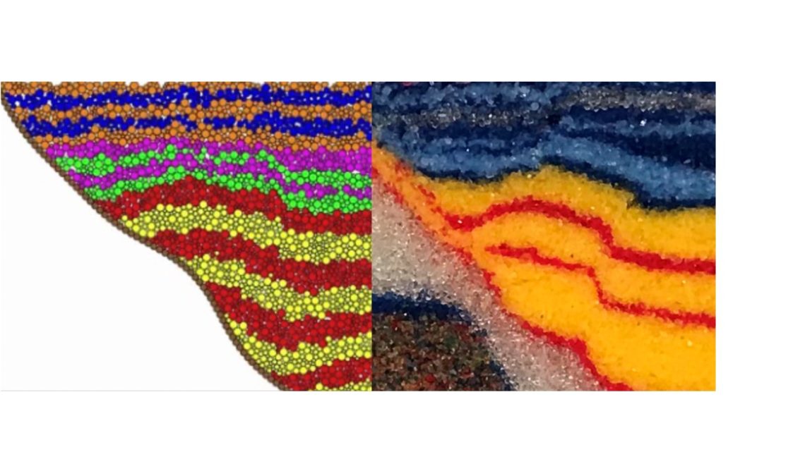
Back in February, I saw several references to the CDEM discrete element modeling tool on Twitter. One of the example simulations reminded me of a “real” sandbox model I made a couple of years ago while experimenting with different material properties. The two results are shown below, with the CDEM example on the left and the real sand model on the right.

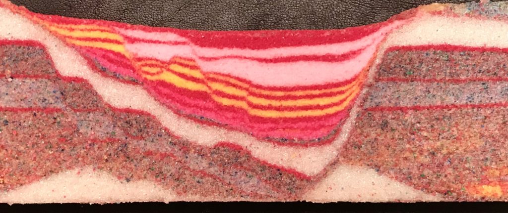
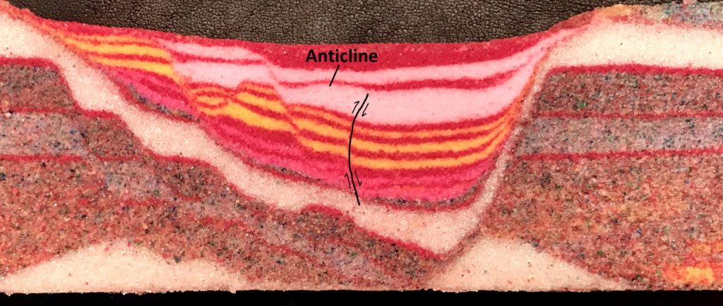
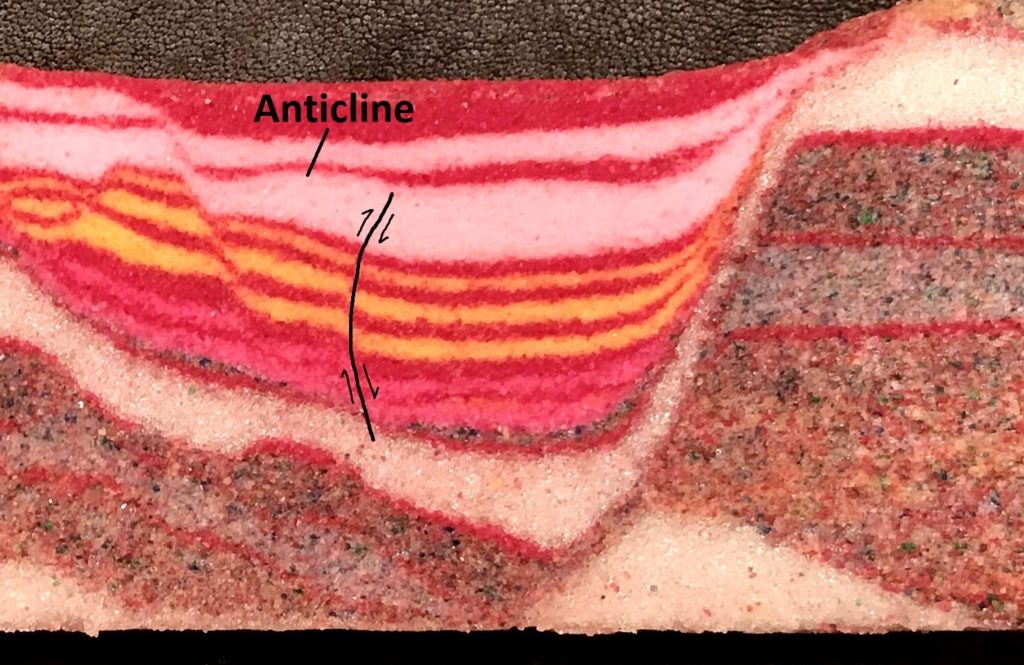
The CDEM example above is the first animation that appears under the Examples tab on the CDEM site. The simulation demonstrates folding above an irregular normal fault, which flattens, then steepens, then begins to flatten again moving downward. The first flattening section causes the formation of the upright anticline, which is an example of extensional fault-bend folding, or rollover. The real-life sand model develops its anticline through the same process, which results from mechanically different layers of granular media within the model.
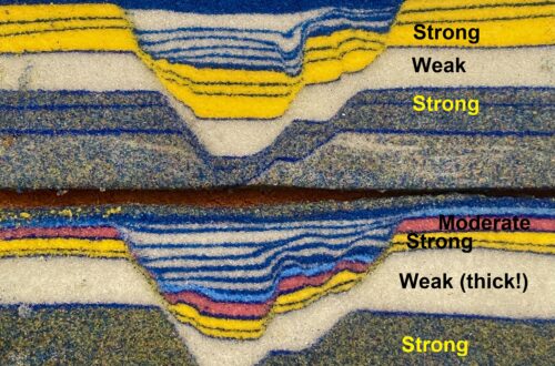
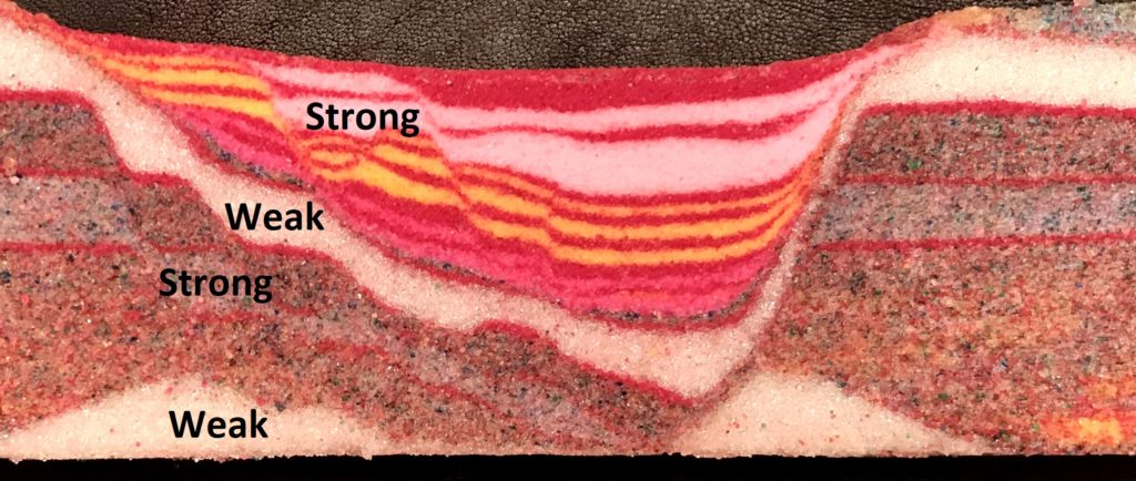
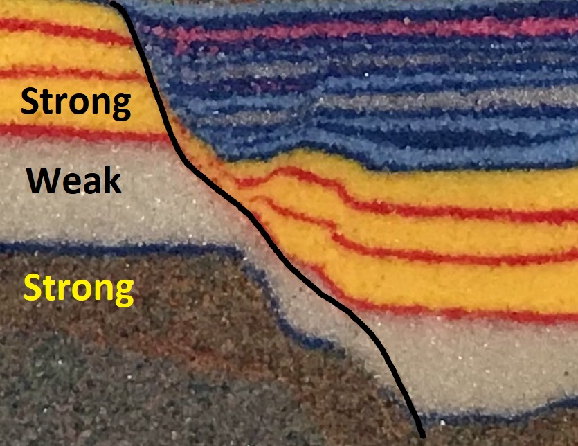
The image above shows a zoomed-out view of the sand model. The upper yellow layers (dolomite sand) are very strong and brittle, as are the deeper gray/multicolor layers (also dolomite sand). The white microbeads in the middle of the model stratigraphy are very weak, and a produce a shallower fault angle than the layers above and below. The resulting fault shape is thus steep-shallower-steep moving downward, which replicates the CDEM model setup. As layers in the hanging wall move over this fault shape, the closed anticline results. The last steepening of the fault also produces the unusual fault to the right of the anticline, which has normal-sense offset deep in the yellow layers and reverse-sense offset at the top of the yellow layers.
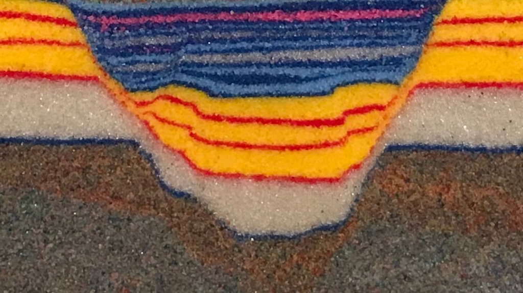
Extensional anticlines reproducibly result from this model setup as long as sufficient contrast exists between different mechanical zones. The images below show two anticlines created with the same microbeads, but faintly different upper and lower units.
Anticlines in these pink-and-green models tend to show small faults or obvious stretching and thinning of layers along the crest of the anticline. This damage results from collapse of the hanging wall onto the flatter section of the main normal fault (sketched and animated in this link). The images below show the position of these faults, which contribute to the ragged appearance of the anticlinal crests in the pink-and green models. These models also developed the normal-to-reverse faults to the right of the anticline, as indicated below. The glare from the microbeads and reflections off of the dolomite sand cleavage surfaces make these models difficult to clearly photograph, but the overall idea is apparent.
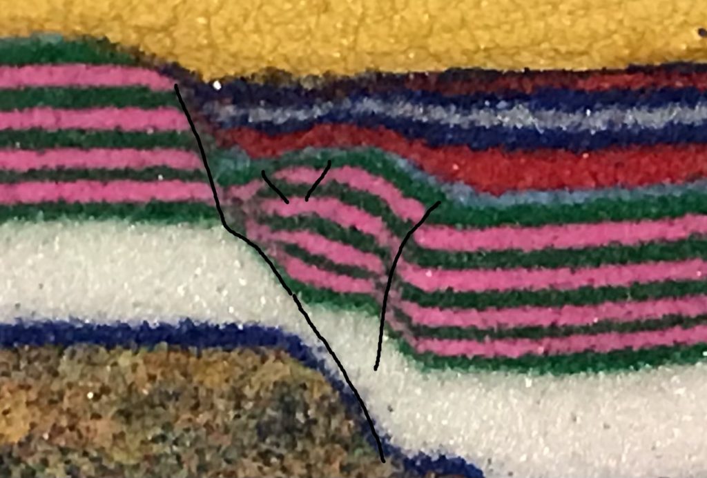
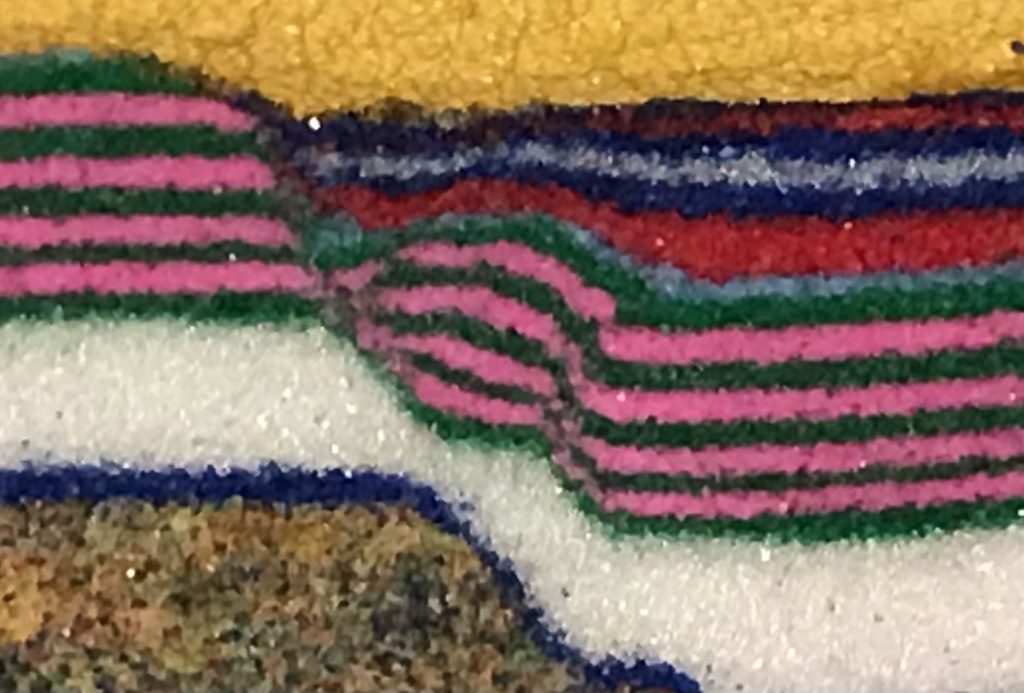
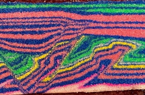
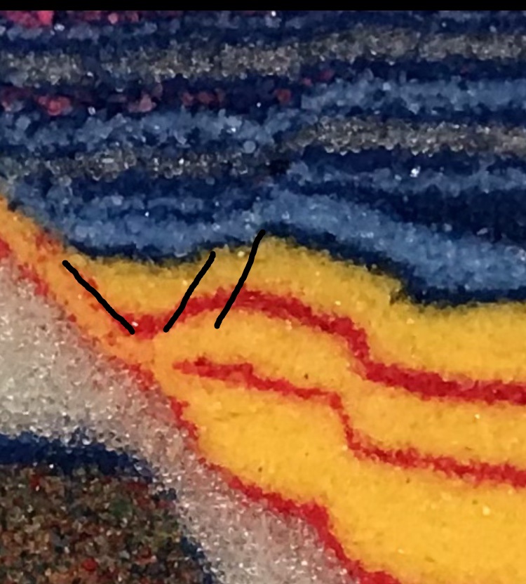
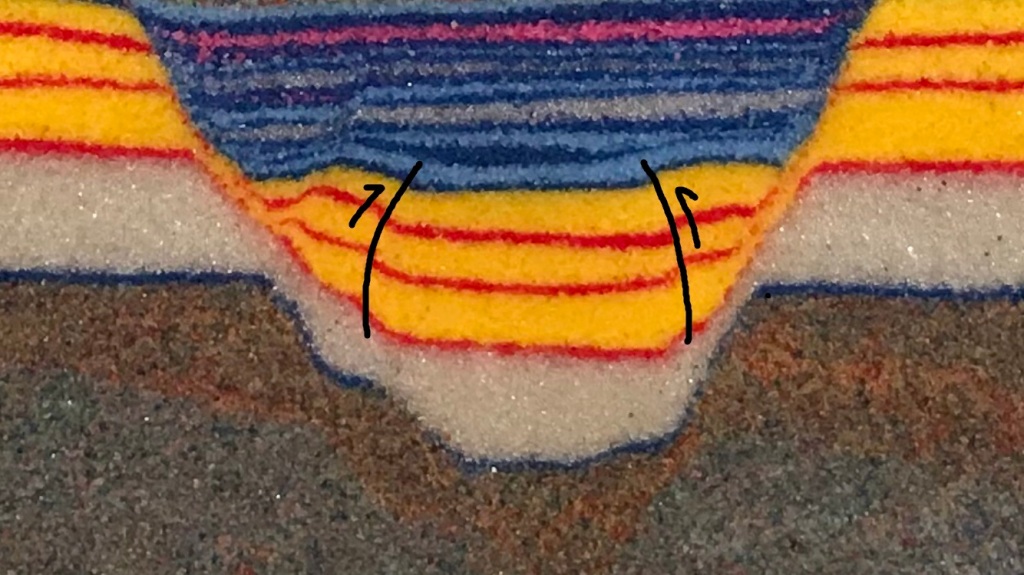
The little faults on the anticline crest are also present in the yellow-and-red model, but are less distinct. When sketched in on the image below, their position is apparent.
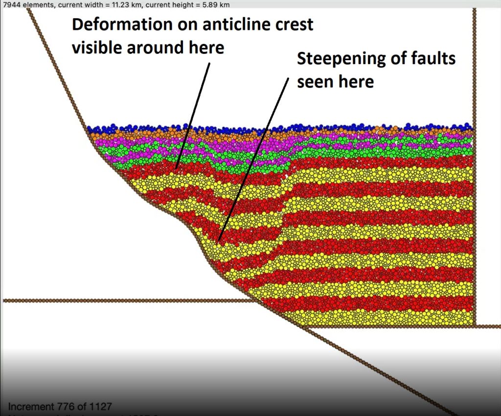
A takeaway message from these real-life sandbox models is that the layers on the anticline crests are not intact and undeformed. Because the anticlines develop from collapse and stretching of the upper layers, deformation and damage affects the layers even though it may not be obvious. Watching the CDEM animation in fast-forward by moving the scrubber bar on the animation video makes this crestal deformation easy to see. The CDEM model also develops upward-steepening normal faults which rotate into reverse-sense motion as seen in the real-life sand models. I have pointed these out in the screen shot below, but the simulation itself is definitely worth a look.
The CDEM animations are mesmerizing to watch, and they provide a great way to visualize changes in the real-life sand models, which I have never been able to produce against a clear sidewall (I make them from a wide sand cake on a table top with a movable base plate). Actually watching areas of focused particle movement in the CDEM animation helps connect initial and final geometries and brings attention to damaged and strained areas, like the anticline crest, that might not receive much notice in the final model geometry. I probably need to download CDEM and play with it myself, but it might significantly impact productivity on other projects!
-
The waddling boulder…a storm-induced trundle* event?
by Philip S. Prince
*yes, trundle will be defined at the end.
I see lots of boulders in the course of my fieldwork, but this one just looked different…
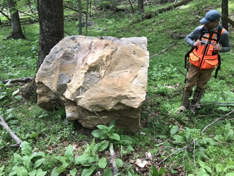
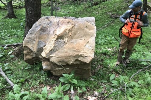
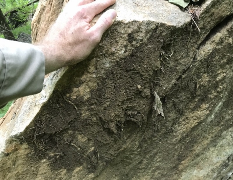
Appalachian Landslide Consultants geologist Aras Mann (pictured above) and I spent a fair amount of time trying to figure out just what made this boulder look so strange. We first noticed its apparently soil-stained color, unusual in its rainy Rutherford County, North Carolina, setting. The boulder also had mud and dead vegetation caked on its corners and edges.
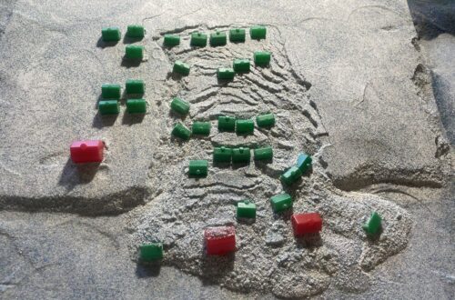
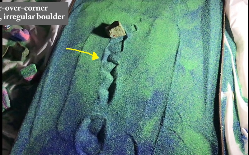
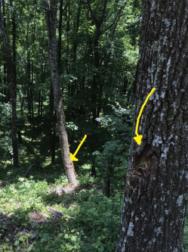
Eventually, we looked towards the slope behind the boulder’s resting place and noticed two flattened saplings and alternating, diagonal gouges in the soil (yellow arrows below) leading down to the boulder. These details made it clear that the boulder had recently rolled into place.
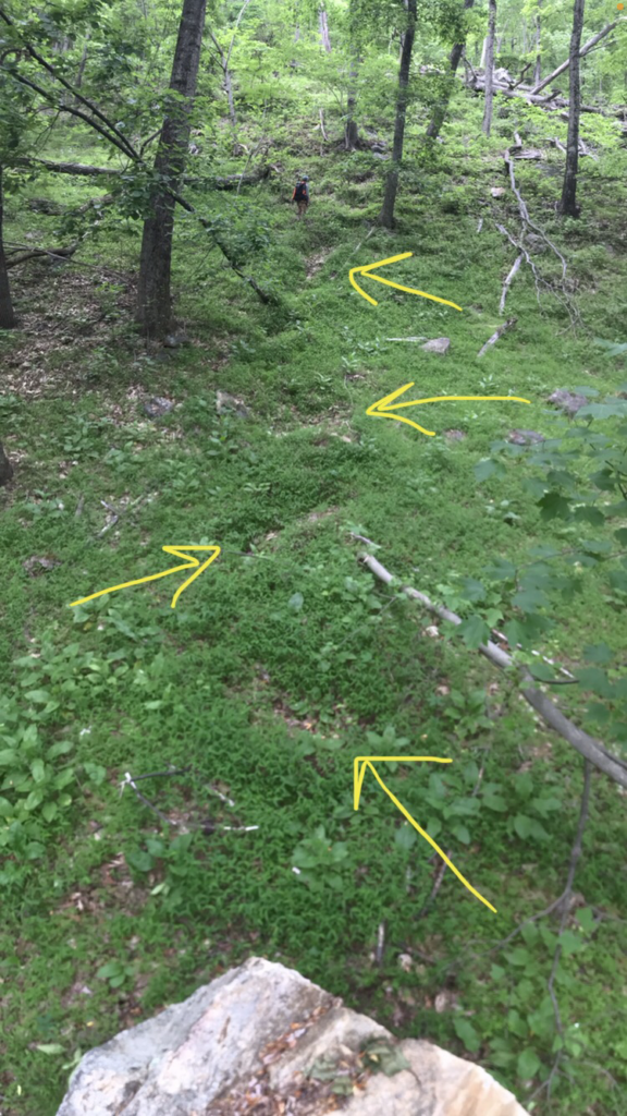
This was (and remains) the first and only boulder I have personally seen that has rolled or tumbled and come to rest recently enough for its track to be visible in the field. I thought the diagonal gouge marks were particularly interesting. For whatever reason, they caused me to visualize a slow, “waddling” rolling style like that of an American football or rugby ball rolling downhill. The boulder had not traveled particularly far across the flat area where it came to rest, and I thought the “waddling” style might explain this.
The boulder had, however, traveled down a significant slope prior to reaching the flat, and should have been moving at good speed. I could not really make sense of the gouge marks, travel distance, and steep slope origin. When I can’t visualize structural geology scenarios, I turn to sandbox models. I tried to do the same here, and I was easily able to produce alternating diagonal “zig-zag” rolling tracks with model boulders and a sand tray.
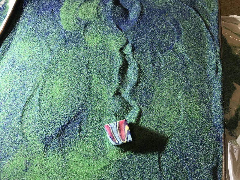
My model boulders were made of dried play-doh, which had been cut into shapes reminiscent of the recently emplaced Rutherford County boulder. I let these roll down a tilted strip of carpet, which caused them to tumble as they accelerated before rolling out across the nearly flat sand tray surface. Tumbling the model boulders turned out to be rather interesting, and was sort of like shooting dice for people that like geology and interesting visual patterns. To summarize the results of dozens of rolls, the model boulders produced either zig-zag tracks from corner-over-corner rolling or longer tracks with a helical pattern from face-over-face rolling. These rolling styles and the resulting tracks are shown in the video linked below (a helical, edge-over-edge pattern is shown in the link image).
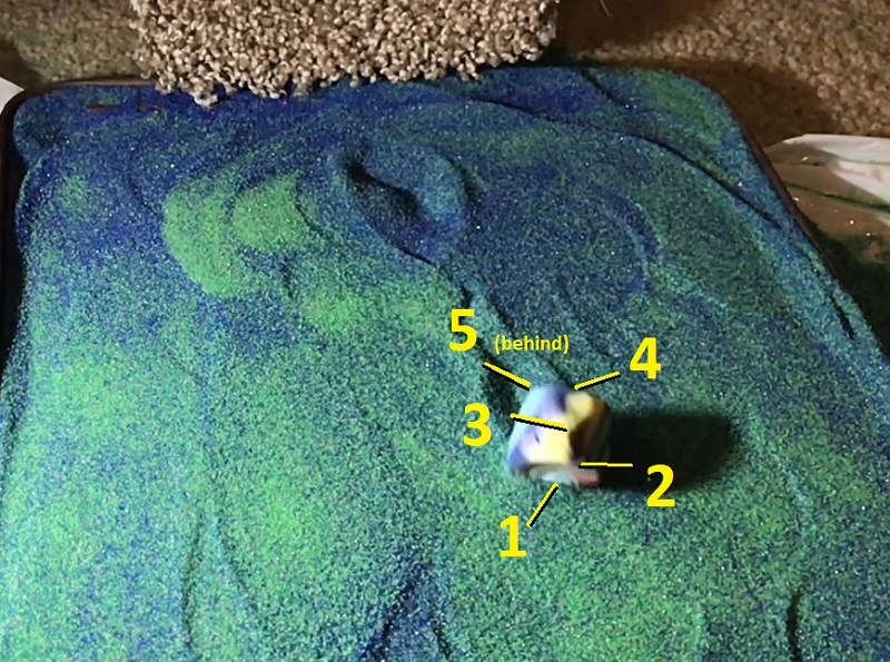
Corner-over-corner rolling occurred when the model boulder did not tumble smoothly down the carpet and thus did not reach a high speed. Once a corner-over-corner roller hit the sand tray, it seemed to lose energy more quickly than the face-over-face rollers, presumably due to the deep gouging of the edges and greater length of the boulder’s diagonal. The image below shows the sequence in which the edges and corners impacted the sand to produce the zig-zag pattern.
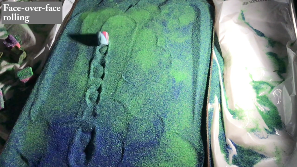
Regular, face-over-face tumbling down the carpet allowed the boulders to reach higher speeds and travel notably farther across the sand tray. The helical pattern (below) results from a slight irregularity in the model boulder’s rectangular prism shape; one edge was slightly rounded.
The models made it clear that the real boulder probably did not make any sort of unusual “waddling” rolling style. Its shape, combined with corner-over-corner tumbling, would have allowed it to make the zig-zag, diagonal gouge marks in its track while rolling in a generally straight line at moderate speed. The corner-over-corner style is a less efficient and sort of off-axis style of movement, but I imagine that to an observer, the boulder would have appeared to simply be rolling at the time of its emplacement.
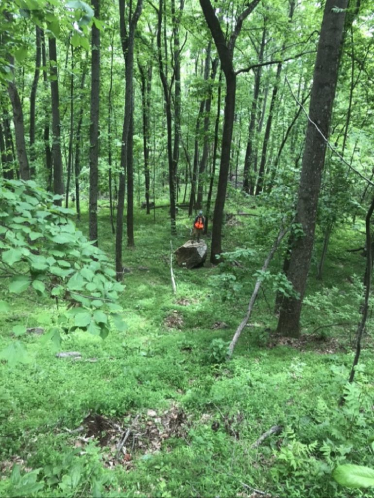
On a later visit to this site, we tried to find the boulder’s place of origin on the slope. The boulder’s track could not easily be traced by impact marks on the slope surface, but scarring on tree trunks made its path quite clear. Corey Scheip (BGC Engineering) examines one of the tree scars in the image below. The dash marks generally show the boulder’s path after the tree impact. It was deflected to the right before continuing downhill to its resting place, shown with an arrow in the darker portion of the image.
The boulder hit several trees on its way down, all of which bore similar scars. The trees were offset in their locations, suggesting the boulder deflected from one to another and followed a Plinko-style path down the slope. The lack of a straight path obviously limited the boulder’s speed and may have prevented it from attaining a faster, face-over-face tumble.
So, where does “trundle” figure into all of this? When I searched YouTube for videos of rolling boulders to try to better understand the origin of the diagonal gouge marks, I repeatedly found “boulder trundle” videos. Apparently, “trundling” is the act of purposely rolling boulders down slopes, often by prying them loose with levers. Limited field evidence still visible during our second visit to the site suggested that the recently emplaced boulder had started rolling after it was pried loose or struck by a falling tree. A tropical depression had passed through the area several months prior, and high winds along steep slopes had knocked down numerous very large oaks. The boulder’s tree scarring and faint slope track appeared to begin just below the base of one such felled oak, suggesting the rolling of the boulder was indeed a natural, storm-induced “trundle.” I’m not sure how often tree fall triggers rockfall in this region or elsewhere, but this scenario has certainly added another element to my own evaluation of possible slope hazards.
-
“Squirrel tail” synclines in the Appalachian Valley and Ridge
by Philip S. Prince
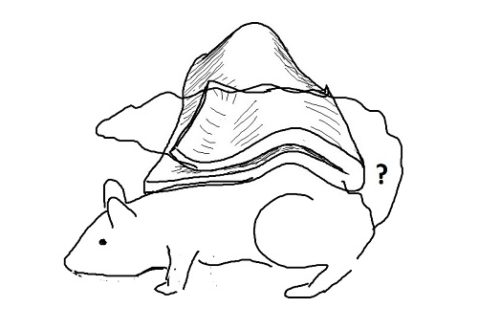
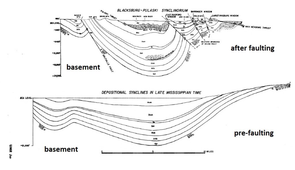
In the course of recent geologic mapping in the Appalachian Valley and Ridge, I came across a great 2010 paper by Jerry Bartholomew and Sharon Lewis describing extremely tight (and ultimately fault-transported) synclines in the footwall of a major Appalachian thrust system. I found myself in need of an analogy to describe the shape of these structures, and I settled on “squirrel tails” because Bartholomew and Lewis’ cross sections of the features reminded me of how a squirrel drapes its tail over its body and head. I am not sure if this is an effective comparison or not, but the overall approach seems to have served humans well when it comes to mentally organizing patterns of stars in the night sky. I provide supporting images below! (nice squirrel photo sourced here).

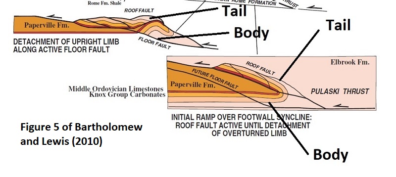
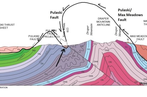
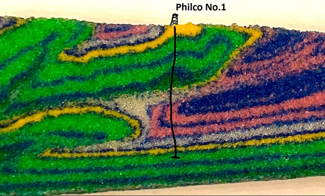
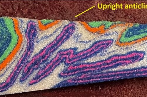
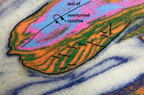
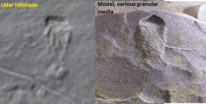
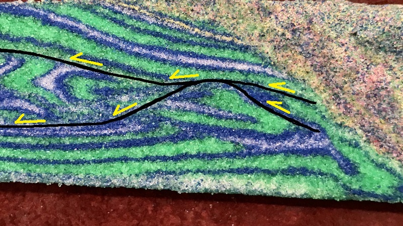
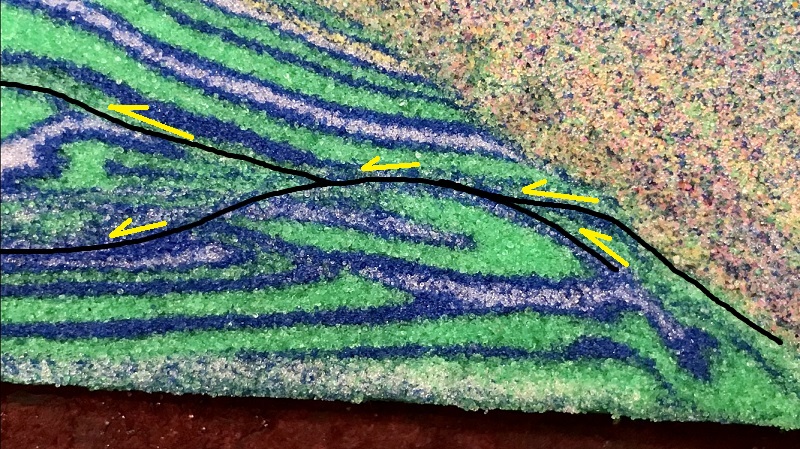
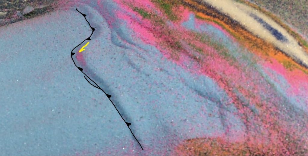
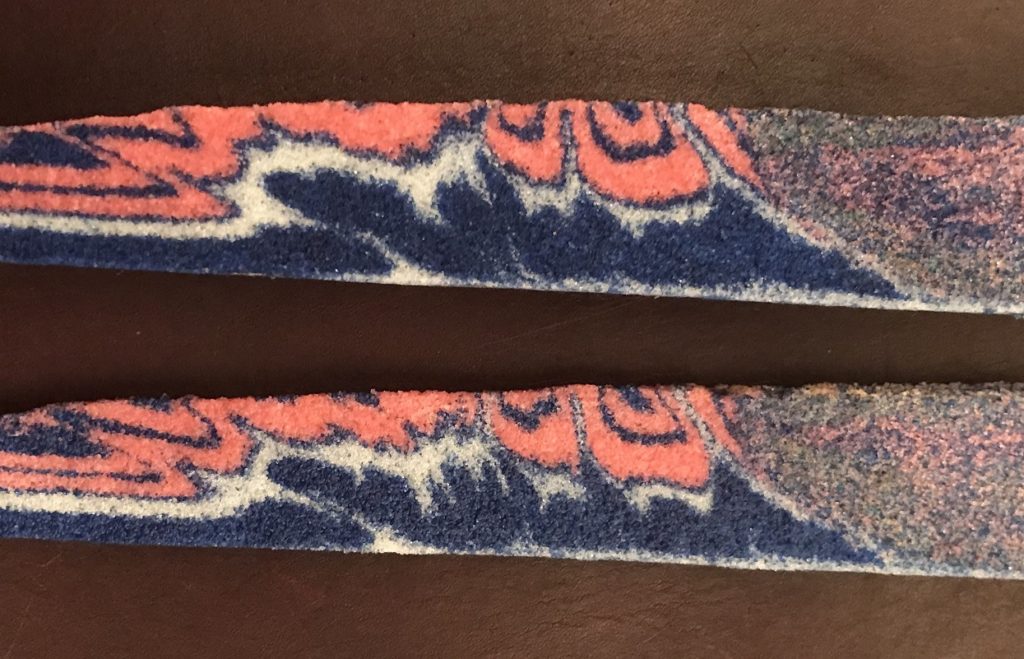
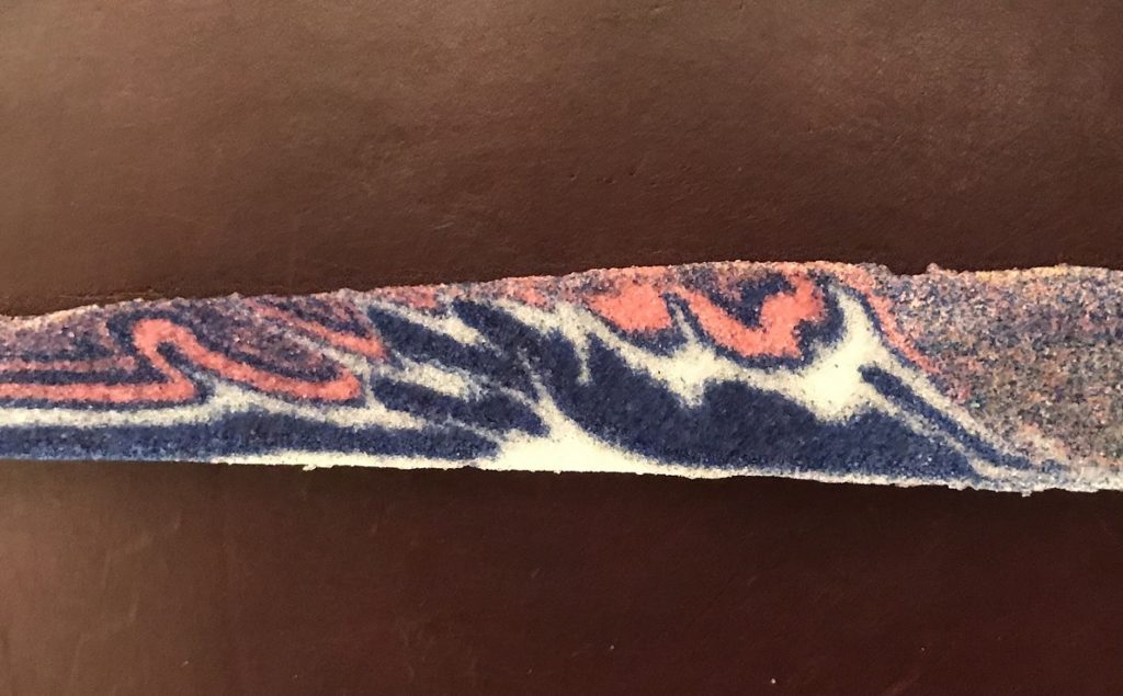
The squirrel tail type locality, which inspired the cross section above, is located between Radford and Christiansburg, Virginia, in the footwall of the Pulaski-Max Meadows Thrust fault system. This structural style came across my radar after I mapped a similar type of structure ~25 miles (40 km) to the southwest, near the town of Max Meadows itself. The geologic map overlay below shows the surface expression of the structure I mapped. Using the squirrel analogy, the overturned area is the tail, with the upright body still below it in the subsurface. The upright body portion is today exposed on Draper Mountain, which is labeled “Upright” below. This area stands out because the blue Siluro-Devonian sandstone unit is effectively folded back on top of itself, with apparently only a thin seam of Devonian shale (dusky blue separating the light blue zones) in between the upright and overturned limbs. The slightly synclinal overturned area is 2,000 ft (630 m) across at its widest, but would have been wider prior to erosion to present-day outcrop level.
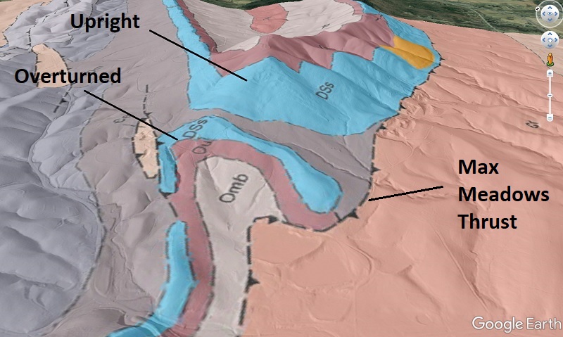
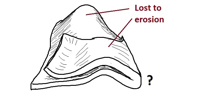
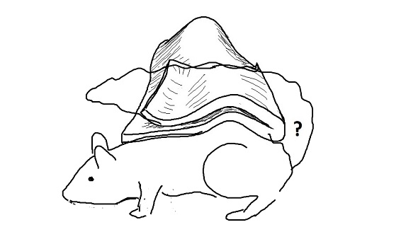
Surface outcrop patterns and lidar-derived hillshade maps suggest the structure of the blue Siluro-Devonian sandstone layer would look something like the sketch below, prior to erosion into its present outcrop pattern. The nature of the hinge area (the “?”–is it faulted?) is unknown. I “squirrel-ized” the sketch in the second image for comparison to Bartholomew and Lewis’ examples. Note that the sketch focuses on only one thin stratigraphic horizon; the pre-erosion structure, as well as the upright limb in the sub-surface, likely involve a bit more section. The Siluro-Devonain layer should also continue in the subsurface to the left/northwest; it is cut off here to illustrate only the folded area.
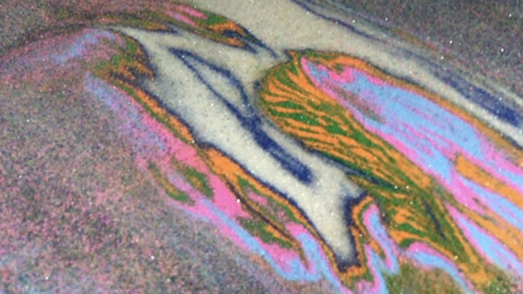
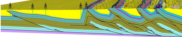
The mechanism through which such a lengthy overturned limb and tight overturned syncline develop is interesting to consider. I tried to create comparable structures in a sand model utilizing several overlapping weak detachment layers (white layers in the model images below). Surprisingly, I was able to produce tight footwall synclines that likely involved a single layer during their formation and initial fault transport. A good example is shown below, along with more squirrel-ization. Yes, this model is hopelessly green. Current supply chain struggles appear to affect colored sand, so only the shape of the structure is the focal point here!
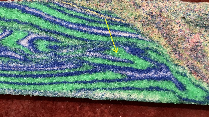
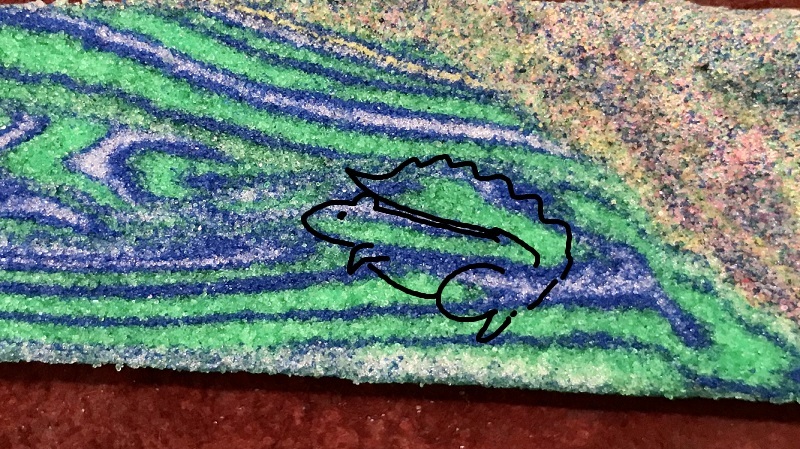
I find this model complicated to look at compared to a nice set of colorful thrust imbricates, but I think it does contain a legitimate squirrel tail-type structure with upright and overturned limbs of comparable length. The limbs are separated by a very small amount of weak material. The structure occurs in the footwall of a major thrust system in the model, which is faintly arched by the underlying squirrel tail block.
I can’t tell you how far the squirrel tail block was transported, as the strata from which it detached began to be thrust back over it as this portion of the model approached the rigid backstop. The right edge of the model also appears to have been damaged by extensional faults as the backstop was removed, but the squirrel tail was fortunately spared. The image below shows a larger view of the model and the context of the squirrel tail block. Its position near the backstop is comparable to that of the real-world squirrel tails, which occur in fairly close proximity to the outermost crystalline thrust sheets of the Appalachian Blue Ridge, which served as backstop to the Valley and Ridge sedimentary fold-thrust belt.
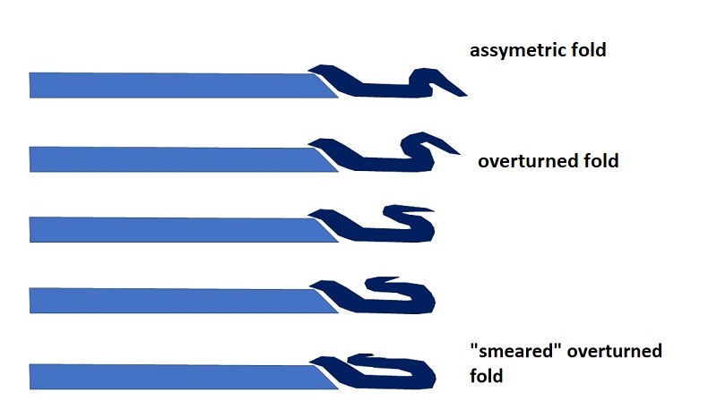
A primary goal of these models was to figure out what the overturning process actually looks like, as the long overturned limb cannot simply swing on a hinge like a door. Based on observations from a couple of other models, I think the overturned limb might develop through tightening and stretching of an early fold at the trailing edge of the future squirrel tail block. The sketches below attempt to illustrate this process. The overturned limb at Draper Mountain is massively damaged (veined and fractured) and only faintly stratigraphically recognizable, and I think the mechanism below would certainly produce extensive damage in the overturned limb.
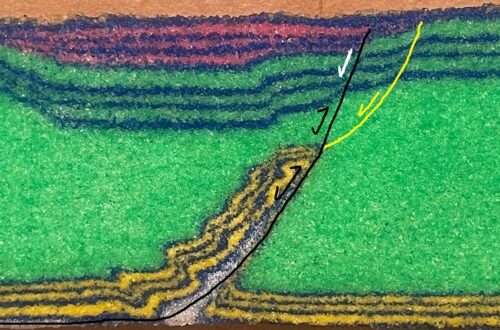
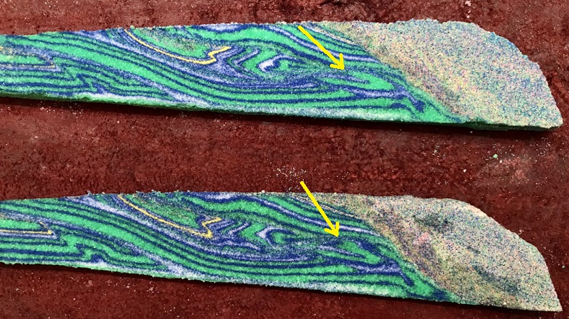
The model below may show the above mechanism in progress. Just below center, a developing squirrel tail is visible, lodged against the the yellow layer ramp (thrust transport was right to left). The overturned tail is not extensively developed yet, and it may show evidence of a tightening and smearing fold set as illustrated above.
I would love to watch one of these features form, but I can confidently say that I am very unlikely to produce one of these features in a model with glass sidewalls. These models also require a large amount of shortening to fully develop, and they rapidly become prohibitively large and heavy due to the volume of sand and microbeads necessary. I haven’t completely abandoned this setup, however, and I plan to try a few more to see what other types of major thrust footwall structures can be developed.
-
Interesting sedimentary basin structures in fold-thrust belt outcrop patterns
by Philip S. Prince
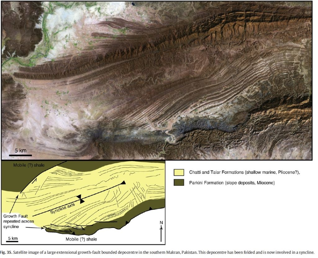
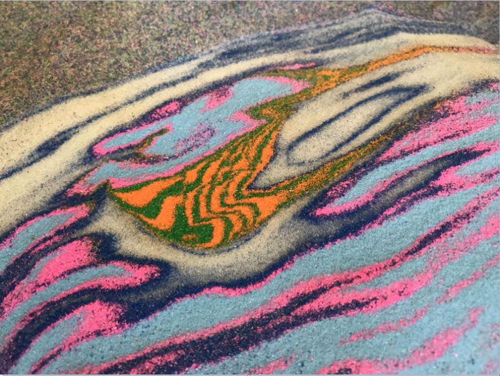
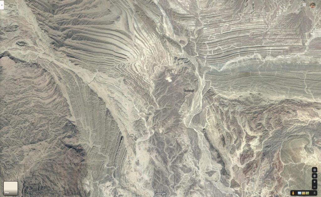
Fold-thrust belts developed in sedimentary rock sequences produce interesting and complex patterns on Earth’s surface. These patterns become even more complex and intriguing when the folded and faulted sedimentary layer sequence contains internal structures that pre-date thrust belt development. A particularly outstanding example of this effect is the Talar Syncline of the Makran fold-thrust belt, in which an extensional growth fault depocenter has been folded, uplifted, and exposed by erosion due to later compressional deformation (see Morley et al. (2011) linked below). The image below is Figure 35 from the Morley et al. paper, showing satellite image of the Talar Syncline along with a conceptual sketch (feature located at 25.458153N 62.205711E).
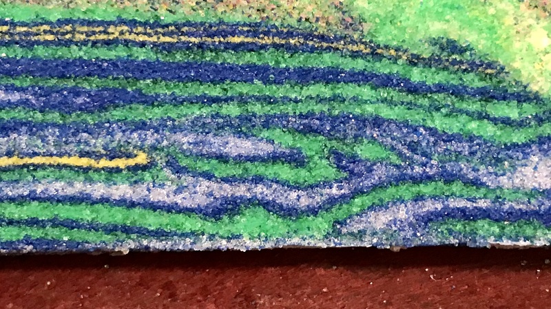
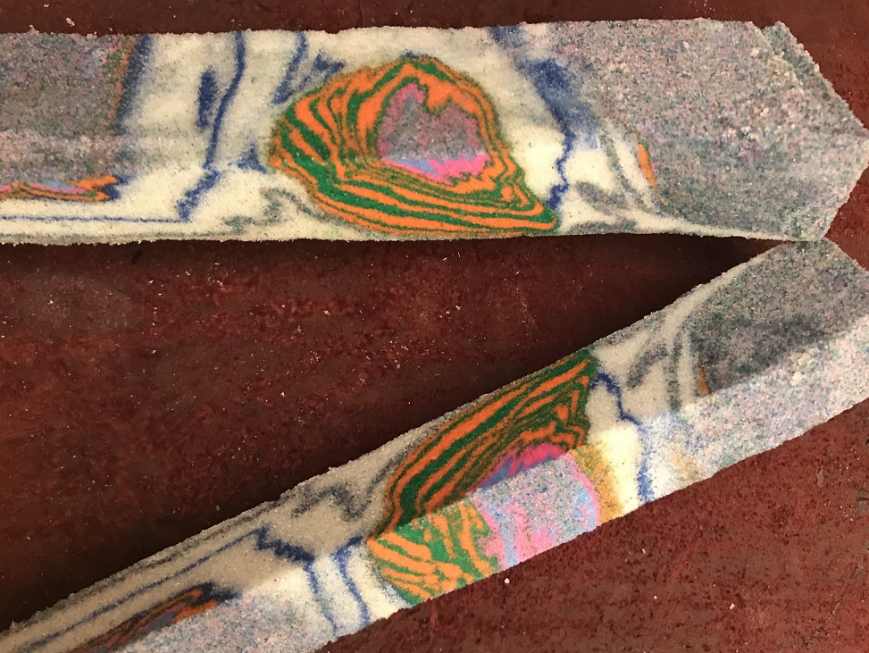
Despite being an incredible example of sedimentary basin and thrust belt process, the details of the Talar Syncline are still somewhat muted in satellite imagery. I tried to produce a sandbox model containing similar patterns highlighted by colored layering. The best model result, shown below. It is by no means a complete match, but it does contain an extensional growth fault-style depocenter deformed by later compressional forces, which bears resemblance to the real thing. Seeing the patterns in the colored model may make the patterns in the real-life, miles/kilometers-wide (and generally brown!) Talar Syncline more visible.
I first read about the Talar Syncline in Morley et al. (2011), and it has been subsequently described in greater detail in Back and Morley (2015), accessible in pre-print here. The Talar Syncline provides geologists a unique opportunity to examine the workings of growth faults and basin fill sediments that are typically buried well beneath Earth’s surface. A closer look at the satellite imagery reveals great exposure of the main growth fault along with several small normal faults offsetting beds within the large-scale syncline structure. The size of the syncline, and thus the scale of the depocenter itself before fold-thrust belt development, is impressive. Because the outcropping layers in the Talar are tilted and not vertical, outcrops widths exaggerate thickness slightly. Even so, everything is big and would be interesting to try to interpret from ground level without satellite imagery. The first image below shows duplexing along the main growth fault; the second is accommodation faulting to the northeast.
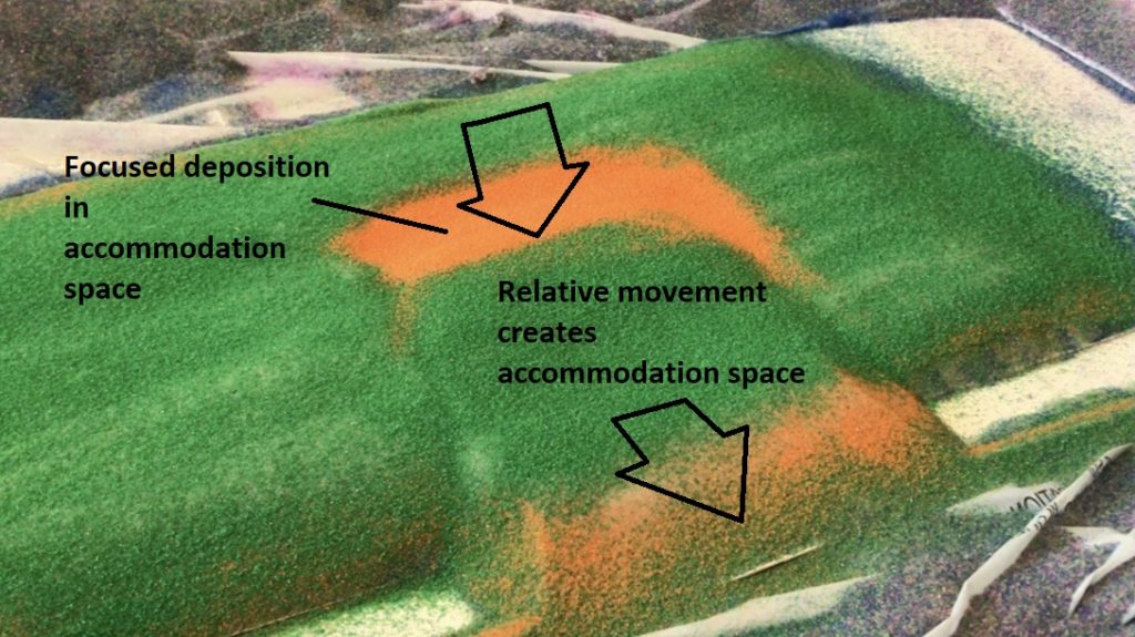
In simplest terms, the Talar Syncline represents a localized sedimentary depocenter folded by later compressional deformation. The model produces a similar structure by using two overlapping base plates, with the upper baseplate containing a cut-out area that will become the depocenter. The upper baseplate is moved relative to the lower baseplate, producing localized extension and accommodation space for more sediment layers. This becomes the locally thick accumulation of orange and green layers with the distinct internal pattern seen in the second image of this post.
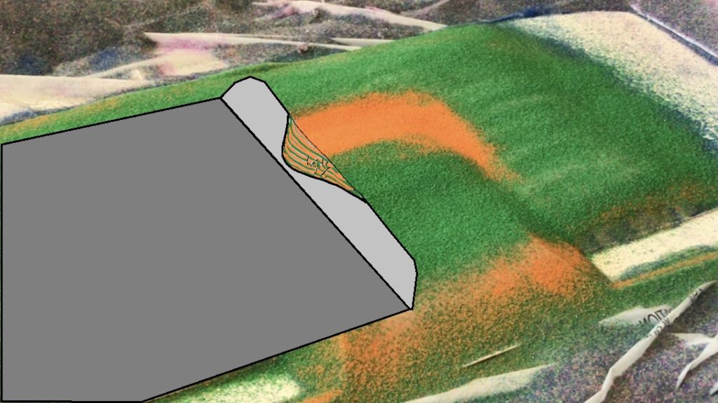
Prior to this movement, most of the layer pack is made of weak microbeads. With addition of frictionally stronger sand to the accommodation space within the microbeads, a depocenter floored by a downward-flattening extensional fault forms. Obviously no cross sectional view is available here, so I have sketched it below.
After deposition of fill, the depocenter is folded, tilted and uplifted during the subsequent shortening of the layer pack. Initial thrust movement of the depocenter is obvious during this phase. The image below shows a broad curve in the thrust front of the model resulting from detachment and early thrust ramp movement of the depocenter.

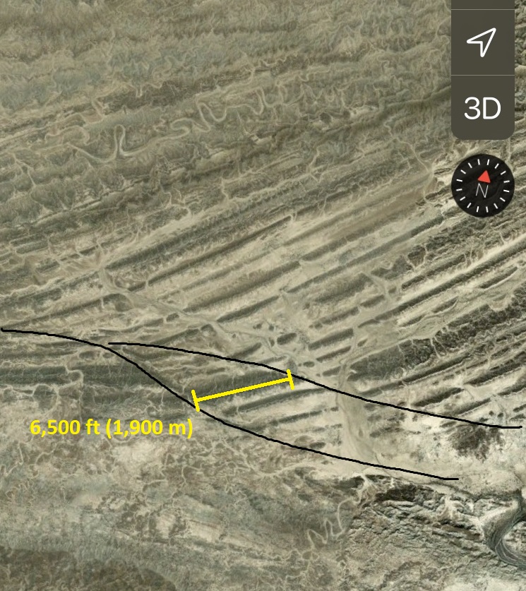
The model was eroded during shortening to counter thickening of the developing thrust wedge. The outlines of the depocenter gradually become visible as the model progresses towards its final appearance, as indicated by the black line in the first image below. The near-final pattern is obvious in the second image.

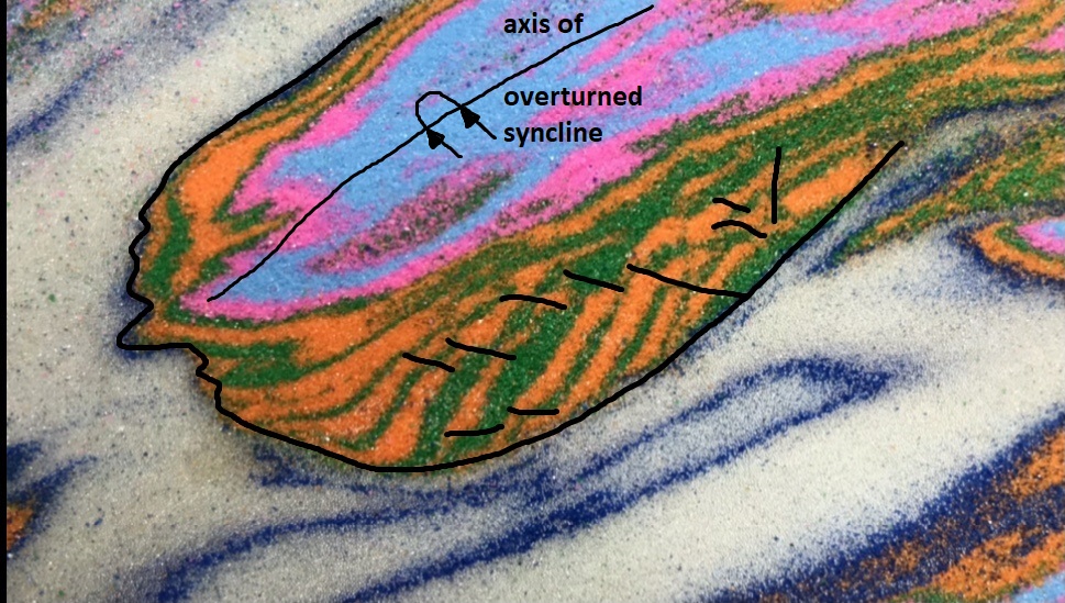
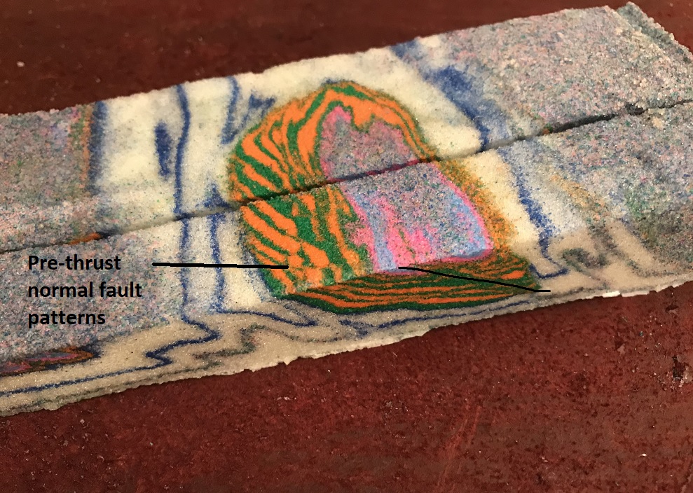
In cross section, the overturned synclinal structure of the depocenter is clearly visible. Away from the thickest part of the depocenter, the overturned back limb of the syncline is displaced along a minor thrust fault. The following images show a map view with extensional, pre-thrust faults and the synclinal axis marked, along with several cross-sectional images.
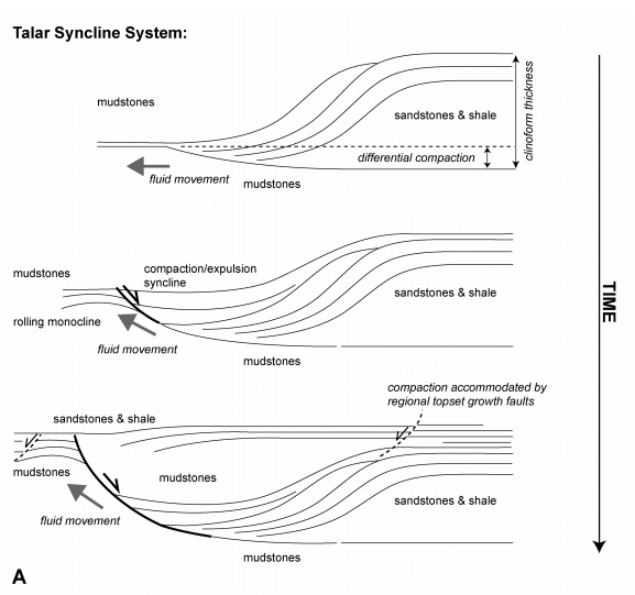
While the model produces a good visual for comparative purposes, it falls short of truly reproducing many details of the real Talar Syncline. The model requires movement of the baseplates to create the depocenter, while the real-life depocenter likely developed due to localized sediment loading atop mobile shale in a large river delta system. The sediment loading gradually pushed the shale out of the way, allowing more and more deltaic sediment to accumulate. This process is conceptually illustrated in Back and Morley (2015).
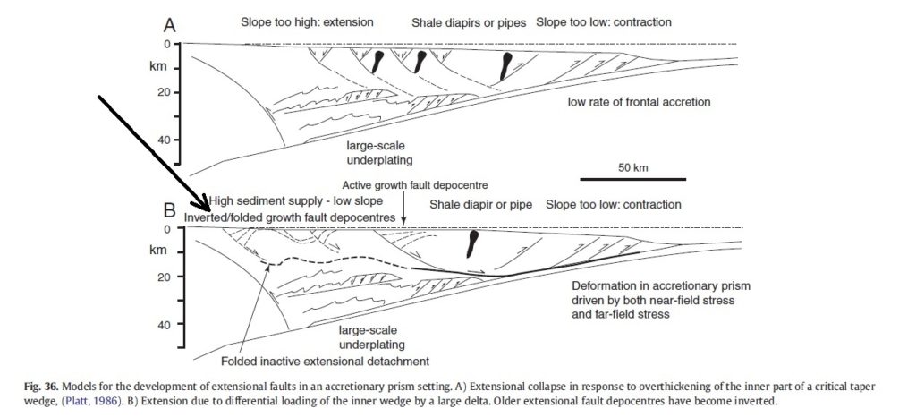
The real Talar Syncline is also much more symmetrical than the model, lacking the overturned back limb. Weaker materials and different ranges of mechanical contrasts would be necessary between the different layers to generate this structural style, and my granular materials just can’t do it. The image from Morley et al. (2011) below shows the position of the Talar and similar structures within the overall Makran Wedge (long arrow).
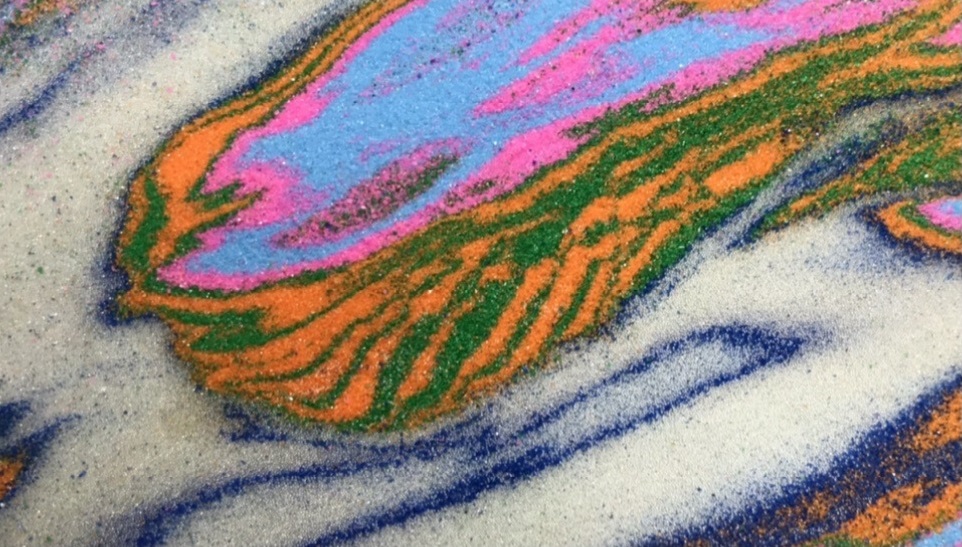
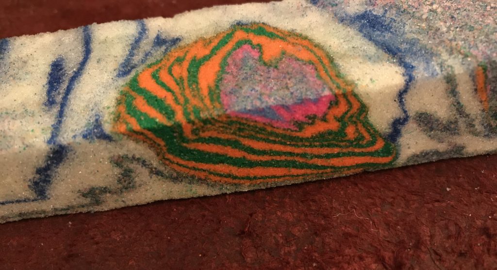
Despite these shortcomings, I was very pleased with the overall model outcome. Subtle changes to pre-depocenter layering, as well as in the layers used to fill the depocenter, resulted in different model outcomes. Two are shown below. In both, the thrusted depocenter is split by an anticline, visible as a dark blue elliptical outcrop ring. The depocenter in the lower image contained weak microbeads itself, and underwent more internal faulting during thrusting. As a result, its overall pattern is less recognizable.

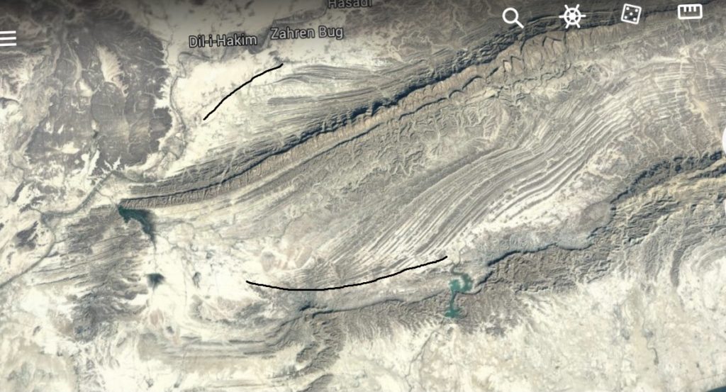
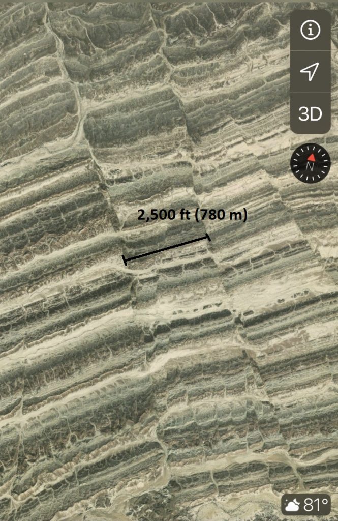
The Talar Syncline is an extreme example of pre-thrust belt sedimentary structures creating unique outcrop patterns, but I am sure it is not alone. Numerous other unusual outcrop patterns exist in this part of the Makran, presumably due to a similar set of formative processes. In the satellite image below, sets of sedimentary layers meet each other at a variety of angles. None of these relationships are consistent with thrust faulting and compressional folding of an orderly, parallel, and uniformly thick package of sedimentary layers. The pattern visible just left of center is particularly well defined (25.947933N, 59.288584E).
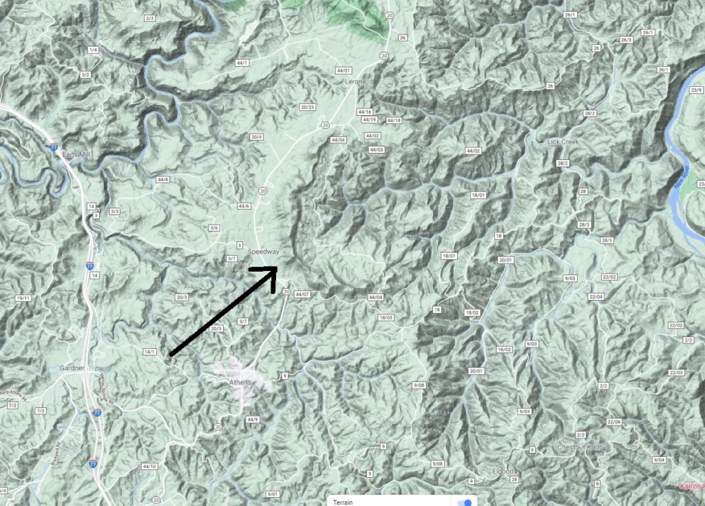
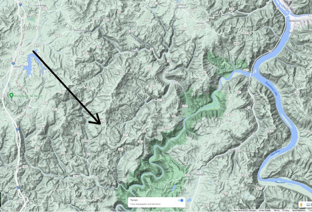
I have always wondered if similar features exist anywhere in the Appalachian fold-thrust belt, particularly in parts of the Mississippian section in eastern West Virginia. Rock type control over topography in sedimentary Appalachia is extreme, so a Talar-like feature should be quite visible if it exists. No such feature is apparent to me anywhere in the sedimentary Appalachians, but a number of unusually rounded and curved drainage and ridge patterns are visible in parts of West Virginia. Perhaps these are expression of pre-fold and thrust depositional structures? Both of the images below are from southeast West Virginia, near the confluence of the Bluestone and New Rivers. The curving ridges indicated by the arrows are a bit unusual within the area. They are located in a broadly anticlinal area, but their curvature and relationship to neighboring topography are not consistent with a solely compressional origin.
-
Central peak formation in model impact craters
Philip S. Prince
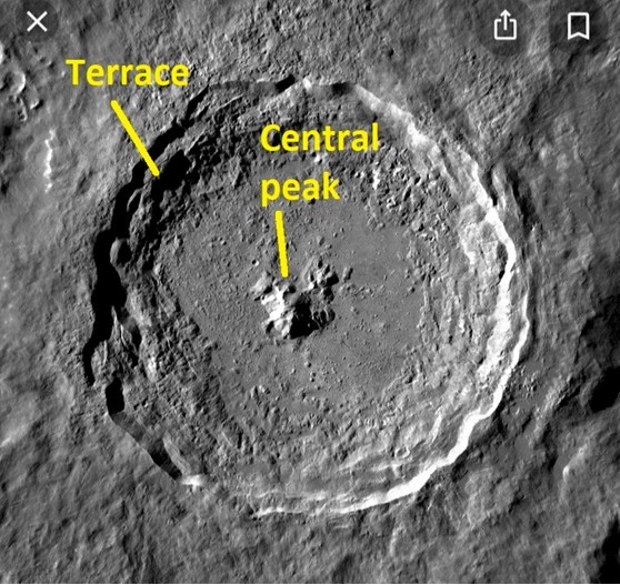
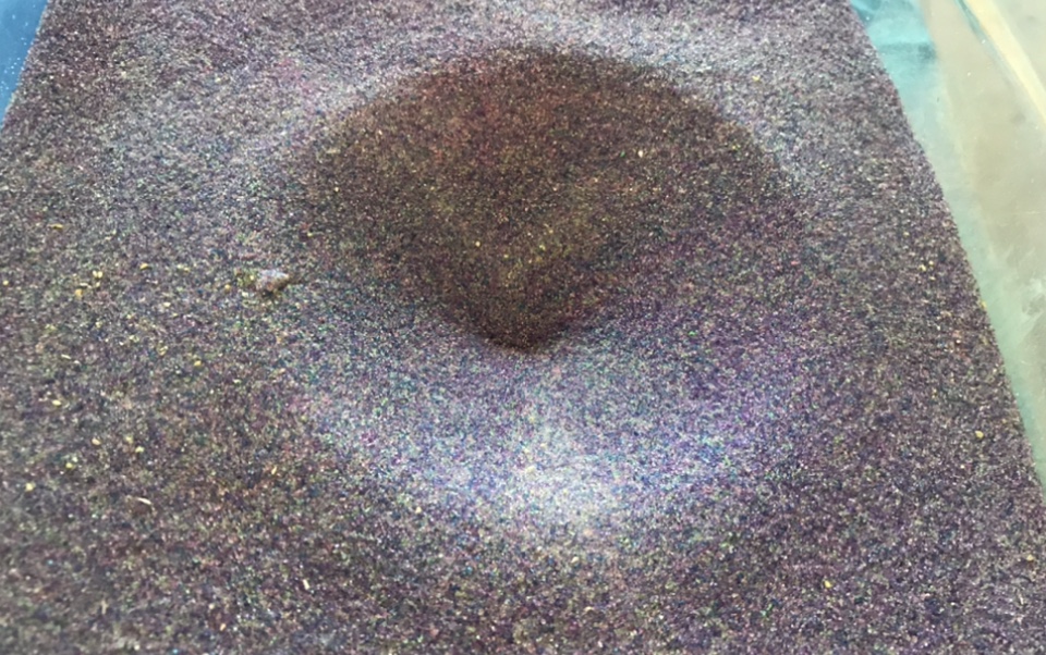
Numerous solid planets and moons in our solar system (our own planet included) host impact craters with conspicuous central peak structures. Lunar crater Tycho, shown below, is a nice example (image sourced here). Central peaks are thought to result from the convergence of inward-collapsing material temporarily forced outward by the impactor, combined with localized unloading of the deeper horizons of the impacted material (see this link). This process can be thought of as the displaced, disaggregated material moving to re-establish equilibrium with gravity, as the walls of the transient crater that forms soon after impact are far too steep to remain stable.
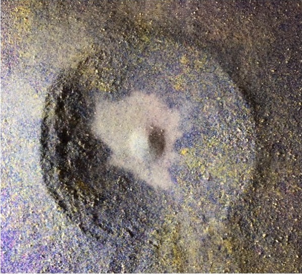
I produced the model impact crater shown below with a combination of the same granular materials I use for tectonic models and a projectile fired from a powerful air rifle (a city-safe version of Gene Shoemaker’s approach at 17:00 in this link). The model crater developed a nice central peak as well as terraced margins. The darker material is quartz sand, combined with a small amount of cornmeal to produce a minor amount of cohesion between sand grains. The white material comprising the central peak is glass microbeads.
The GIF below shows the formation sequence of the model (a YouTube video is linked at the end of the post). The central peak is not unlike a “splash” of granular material that develops as material displaced by the impact collapses back into the crater void. When frictional contact is disrupted by the accelerations and void produced by the impact, the material is significantly weakened and temporarily behaves more like a fluid moving to re-establish gravitational equilibrium. The base of the early crater void (or transient cavity) is also unloaded with respect to the surrounding intact layer pack, and some of the initial peak growth may result from in-place material being pushed inward and upward by the surrounding load.
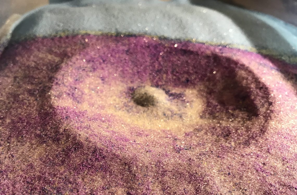
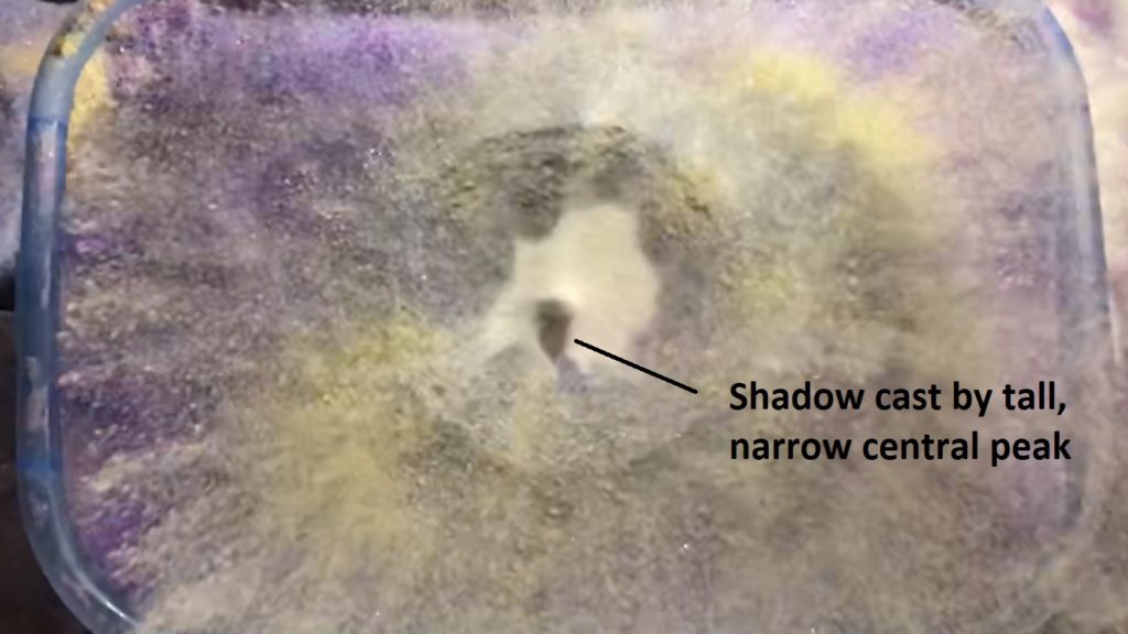
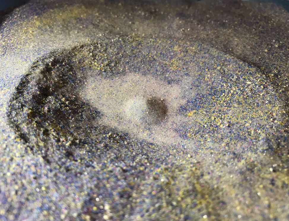
An interesting detail of this model is the temporary (transient) height and shape of the central peak. Its shadow reveals that it attains a very tall, narrow, and definitely splash-like geometry before collapsing to the angle of repose of the granular material (glass microbeads). The frame below shows the central peak at it maximum height and associated highly unstable shape. Ejecta is still spreading outwards at this point in the experiment.
The final, stable central peak is much shorter and wider, with its geometry reflecting the frictional strength of the microbeads.
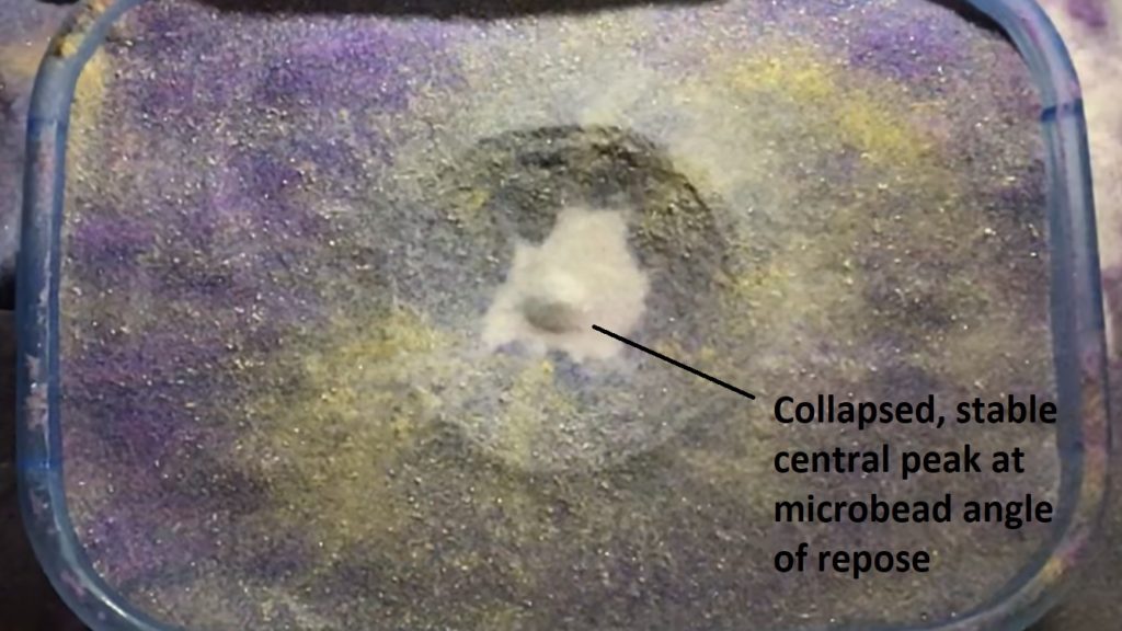
The peak is only a fraction of the height of the inner crater wall.
Central peaks are composed of material derived from deeper below the surface than their surroundings. The following set of images shows a deeper gray layer beneath the white microbeads that is brought to the surface in the central peak. Because these models rely on material properties to produce the central peaks, the introduction of too much colored sand into the microbead zone will prevent peak formation.
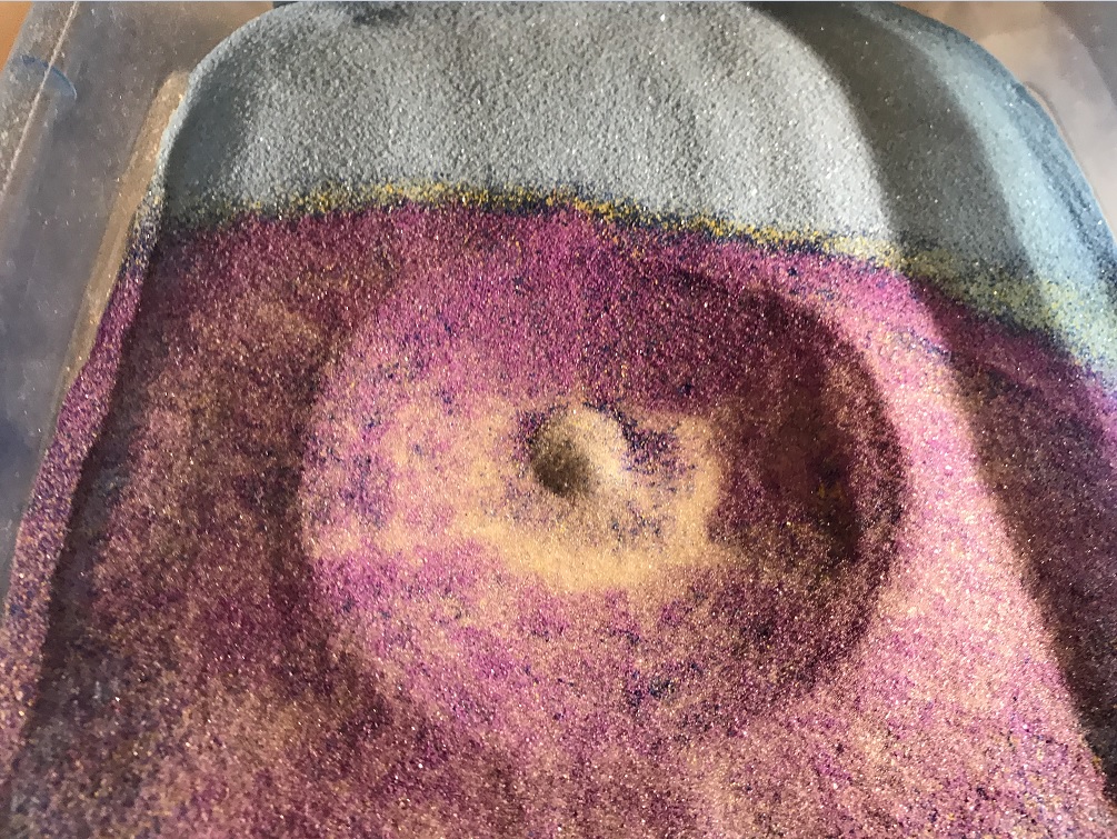
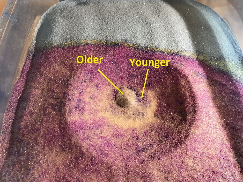
The models shown above were produced with a nearly vertical impact. The material that produces the central peaks in these models tends to rise in the direction of impactor origin. A more angled impact produced a slightly off-center, elongated peak.
In this case, the central peak material, from deeper in the layer pack, ends up on top of younger material (purple) that slumps in from the crater walls. The image below is oriented as if looking from right to left in the GIF above. This experiment also produced nice terraces, one of which is highlighted by shadowing (right side of crater).
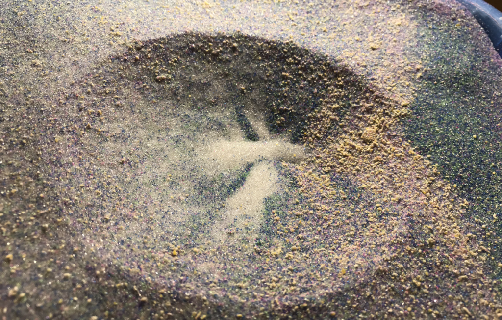
An extremely low-angle impact (20 degrees above horizon or so) produces the same style of response in the layer pack. In this case, however, the “splash” of material is directed back towards the low-angle origin of the shot, producing an elongated zone of material that does not rise noticeably above the crater floor. The older material drapes across younger layers that were tilted backwards towards the impactor’s origin.
This crater was only faintly egg-shaped (see below), despite the angle of approach of the impactor and the hugely asymmetrical wave of ejecta.
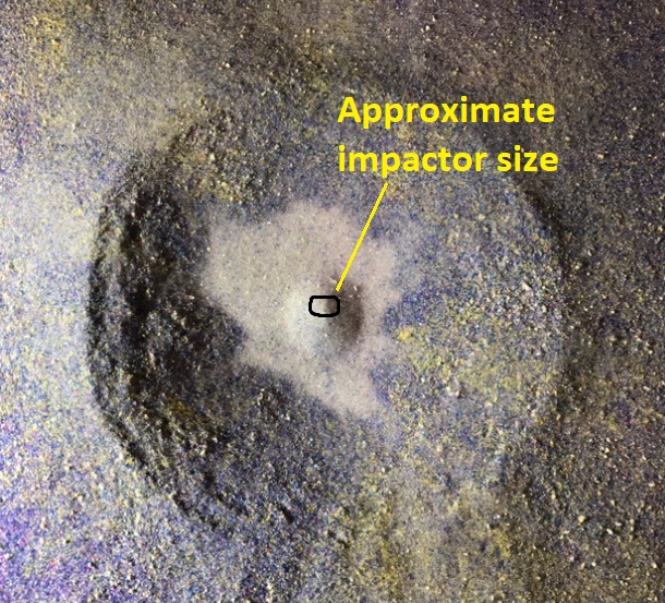
I gave these models a shot (pun intended) in response to a viewer comment on my YouTube page. The models were set up to produce the central peaks using a weak and non-cohesive material (the white microbeads), in contrast to the wet, highly cohesive sand suggested in the viewer comment. I selected and layered the materials (weak microbeads under stronger, more frictional sand) to produce the desired result. Presumably, the greater strength of the outer, more frictional sand layer focuses response of the disturbed material into the weaker microbeads, which respond dynamically due to their lower strength. Shooting a mechanically homogenous (all sand or all microbeads) material with the same impactor at the same velocity produces a crater with no central peak. The crater walls steadily slope towards the crater’s center, as seen below.
In any geologic model, assumptions have to be made and scaling issues will always be present, and these conceptual crater experiments are no exception. The microbeads are slightly less dense than the overlying sand (2.5 g/cc vs 2.65 g/cc), which is the reverse of density relationships that should be present on solid planetary bodies (relevant if the impact effects are sufficiently deep to cross material boundaries). The beads are also weaker than the overlying sand, in the sense that their round shape results in less bead-to-bead frictional coupling. In the real world, rock masses of comparable composition should be stronger with depth due to increasing confining lithostatic pressure, unless thermal or fluid pressure effects disrupt this relationship. Impactor velocity and behavior is also an issue, with the impactor’s intact survival of the impact and its speed (250-300 m/s or so) being questionably scaled. The models shown here do, however, generally represent a style of material movement that is thought to be the principal contributor to central peak formation. Elastic rebound of deeper horizons is also thought to be a component of central uplift in craters, but I do not think it is noticeably represented here.
Various approaches can be used to reproduce certain characteristics of impact craters, though no single method is perfect. Even simple experiments can still be usefully representative. High-velocity projectiles and minimally or non-cohesive sand are effective in producing large craters relative to projectile size, as well as for demonstrating the influence of impactor flight angle on crater shape. Even though the energy in the air rifle projectiles used here is modest compared to Gene Shoemaker’s rifle round, craters are still quite large relative to the impactor itself.
The model shown in this link uses a lower-energy, much larger impactor with a very detailed model setup to replicate ejecta ray patterns. The crater produced is not much larger than the impactor itself. The modeling approach here is entirely different, but it is still effective in proposing a mechanism for a distinct and well-represented detail of real craters.
Videos of the experiments shown in this post, along with a couple more, are available at the link below:
-
The Ray Sponaugle well: A 13,000 ft lesson in Appalachian Valley and Ridge structure
by Philip S. Prince
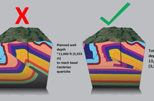
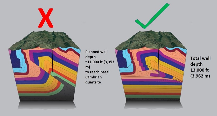
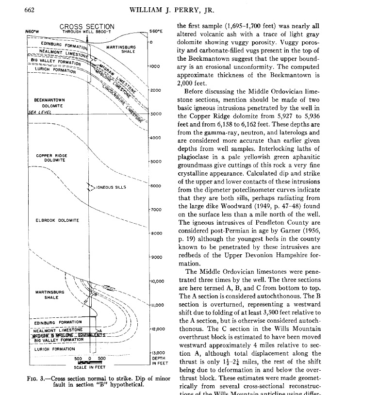
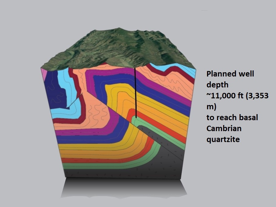
The 1964 Ray Sponaugle #1 well of Pendleton County, West Virginia, did not produce any hydrocarbons, but it did provide essential information about the structural details of a major Appalachian Valley and Ridge anticline and sedimentary fold-thrust belts in general. The well was intended to target lowermost Ordovician- and upper Cambrian-aged carbonate layers beneath the Wills Mountain Anticline, a major structure at the leading edge of the zone of significant folding and faulting in the Valley and Ridge. The well was expected to terminate in Cambrian quartzites at slightly less than 11,000 ft (3,353 m) below the surface.
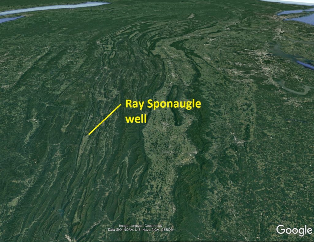
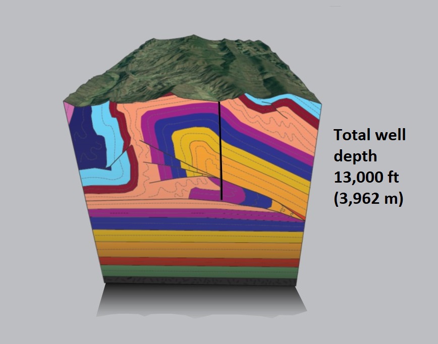
To the surprise of the drillers and geologists involved with the project, the well bore never got anywhere close to the Cambrian quartzite. At 10,000 ft (3,010 m) below the surface, the well passed through a thrust fault and entered a tight, nearly recumbent syncline cored by the same Ordovician shale unit into which drilling began. Ultimately, after 13,000 ft (3,962 m) of drilling, the well was terminated in a horizon of rock equivalent to layers the well first passed through only 1,300 ft (396 m) below the land surface. The block diagram below shows this basic structure; the heavy black vertical line is the approximate well bore. The basal Cambrian quartzite layer (green) was probably 8,000 ft (2,438 m) or more below where drilling stopped. Pre-drilling understanding of Valley and Ridge structural style was obviously a bit off target…
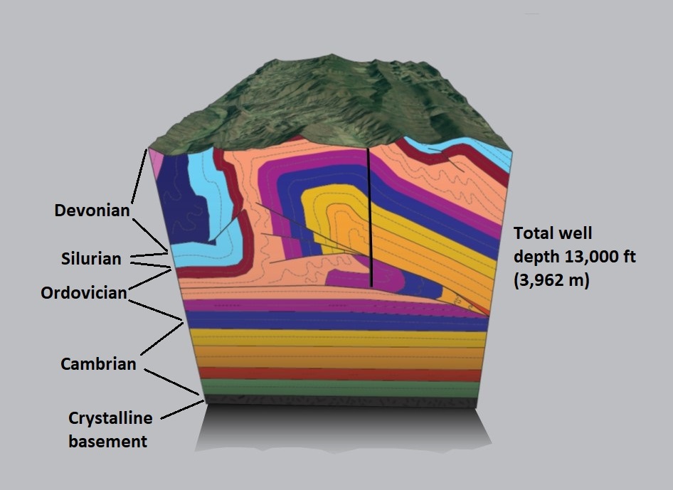
I drafted this block diagram from Google Earth surface imagery, a partial cross section from William A. Perry, Jr.’s 1964 AAPG Bulletin article describing the well, and Kulander and Dean (1986). The purple layer is the Middle Ordovician limestone interval through which the well bore passed near the surface and ultimately terminated in at 13,000 ft total depth. Perry’s description of the well, accessible here, is a fascinating read, and one can genuinely sense his surprise at the outcome, largely due to drilling so far to reach the same rock layers the well passed through much closer to the surface. Perry’s small cross section from the paper is shown below.
While the geometry shown in this cross section and in the block diagram would be considered a very reasonable Valley and Ridge (or any “thin-skinned” sedimentary fold-thrust belt) structural style today, conceptual models of Appalachian Valley and Ridge geometry were somewhat different in 1964. Drilling was expected to encounter the Cambrian quartzite (green in the block diagrams) at just under 11,000 ft (3,353 m) deep because faulting beneath anticlines was believed to involve crystalline basement rock (gray in the diagrams) and cut across sedimentary layers at constant angles, regardless of the mechanical properties of the layers. I tried to re-work the block diagram to illustrate this prediction, basing the geometry on some papers from the time.
Compared to the actual structure revealed by drilling, the source of Perry and others’ surprise is evident:
The Sponaugle well showed that faulting could localize within (and propagate parallel to) weak shale layers, allowing portions of the sedimentary section to detach, fold and fault above and independent of the basement rock. Faulting did not cut through the entire section at a fairly constant angle all the way down to crystalline basement (see the Cooper section at the end of the post). The structural style revealed by the Sponaugle well also provided a way to account for rock volume inside of anticlines by stacking and repeating large, shale-bounded portions of the stratigraphy without using basement rock and the full sedimentary section moving together. Perry rightfully deemed it necessary to reconsider Valley and Ridge structure at all levels. This was one of many steps towards the adoption of the “thin-skinned” model for the Valley and Ridge, in which major thrust faults sole into a Cambrian shale decollement (detachment) and step up into younger shales, independent from deeper Cambrian units and basement rock. Analogous thin-skin style geometries can be replicated in physical models containing weak layers to serve as decollements.
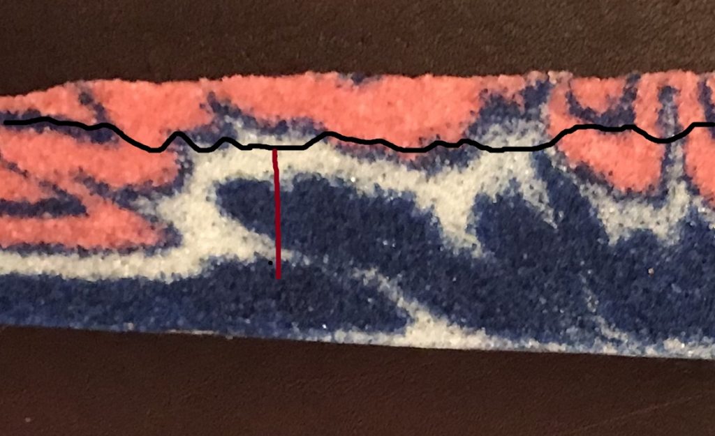
In the model above, the white layer at the base of the section is the master decollement, representing the detachment between the layer pack and the fixed base on which the model was produced. The mid-section white layer will also develop very low angle, nearly flat fault segments that connect steeper faults cutting the blue and pink layers. Working together, the two weak white layers allow the blue layer to be stacked on top of itself. A well drilled in the center of the frontal anticline (maroon line) from an imaginary land surface (black line) would pass through structure comparable to Sponaugle. The frontal anticline containing the doubled blue layer is quite broad, which might suggest it involves a great thickness of layers. Instead, doubling of the blue layer accounts for the large volume of material inside the broad anticline. The full model, and another section from the same experiment, are shown below.
With two weak layers and localized erosion above a growing anticline, the stacking can be taken to extremes as seen in the model below.
The Sponaugle well was just one of many drilling enterprises that ended up informing interpretations of the Appalachian fold-thrust belt and many other thin-skinned sedimentary fold and thrust belts around the world. Today, structural interpretations in these settings place great emphasis on relative rock strength and anticipate zones of flat decollement faulting in shale or evaporite layers. These flats can later be deformed by subsequent faulting, creating great structural complexity. The Bolivian sub-Andes section below from Rojas Vera et al. (2019) is a good example (it is reflected to match the transport direction of images above). The anticline at the center of the image is architecturally similar to the Wills Mountain structure revealed by Sponaugle.
While Perry’s 1964 cross section would be well-received today, he was going out on a limb at the time. When the Sponaugle well was drilled, the basement-involved model for Appalachian structure was deeply entrenched. A particular champion of the model was Byron Cooper of Virginia Tech, who outlined his thoughts on Valley and Ridge structure in a 1968 paper available here. A cross section from Cooper’s paper is shown below, with several faults continuing down through sedimentary layers into basement as initially expected for the Sponaugle drilling site.
This now-disproven perspective on Appalachian fold-thrust structure centered around subsiding synclines and forces internal to the folded and faulted area, bearing some similarity to models of “wrinkle ridge” formation in lunar/planetary craters. Notably, Cooper wrote the paper containing the section above in 1968, four years after the results of the Sponaugle well were published. He chose to omit Sponaugle and other wells in Pennsylvania from the paper as they were not consistent with his favored model. Cooper’s work was based largely on outcrop observations, however, and additional drilling- and seismic-based studies from the Valley and Ridge continued to reveal details its thin-skinned architecture during the 1970s and 1980s. By 1985, thin-skinned, decollement-based structural models had been developed throughout the Valley and Ridge that are still used today and remain conceptually, stylistically, and geometrically valid.
-
Normal fault, reverse fault, or both?
Philip S. Prince
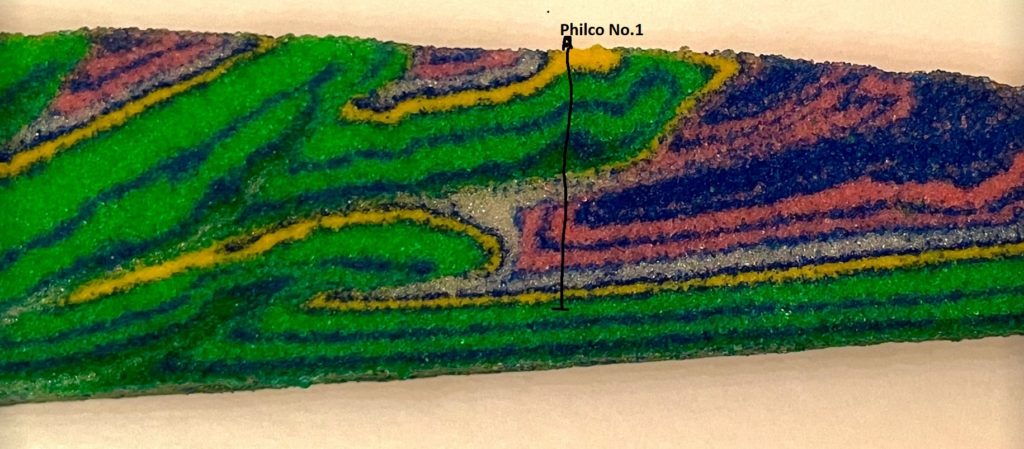
This model serves as a follow-up to a an earlier post about small reverse faults that form in a model subjected only to extensional movement. I wanted to try to produce similar faults in the sediment package added to the growing basin in an extensional model; the original model formed the interesting faults in the pre-extension layers. The new model, whose color scheme is admittedly quite shocking (think Pepto-Bismol bottle), is shown below. The interesting fault is at the center of the image. The fault is traced in black in the lower image, with arrows indicating movement sense.
In this case, the fault in question appears to simultaneously accommodate normal- and reverse-sense motion. Layer offsets are normal-sense, like the other faults in the model, in the deeper portions of the fault. Offsets are slightly reverse-sense in the upper parts of the fault, although the dip of the fault is extremely steep and offset is minimal.
This model was not made in a clear sidewall box (I don’t think the fault in question would even form in one), and the surface of the model during deformation does not provide much insight into how the fault moved and when. Some indication of the reverse-sense movement was apparent on the model surface, but the bright colors of the layering prevented it from showing up in photography. I think a very generalized explanation of the unusual fault is that the large block of layering which it cuts is adjusting to being “packed down” into the narrowing basin. This adjustment is a product of the differing strengths of the materials used and their ordering in the stratigraphy, which control the dip of the main normal faults in the model.
The pre-extension weak layer immediately above the gray “basement” is key to developing the unusual fault geometry. Normal faults cutting upward through the basement flatten as they pass through the weak layer, creating an unusually wide block of material that subsides with continued extension (see the fault-propagation fold animation in the earlier post). As the wide block of material is forced to adjust to the downward-narrowing basement walls, it folds into a syncline and locally creates mild compression due to the thickness of the block. The “normal and reverse” fault thus behaves almost like a hinge, which accommodates the flexure of the subsiding block to fit the basin margins.
The original post mentions descriptions of real-world examples of unusual faults like the one discussed here, so it is indeed a feature observed in nature. From an interpretation standpoint, I think I might find the reverse-sense movement and adjacent anticline very confusing. These features might be thought consistent with the onset of compression and inversion, but they can develop entirely through extension if the different rock strengths allow normal fault dips to vary with depth.
-
Interesting Reverse Faults in a Simple Extensional Sandbox Model
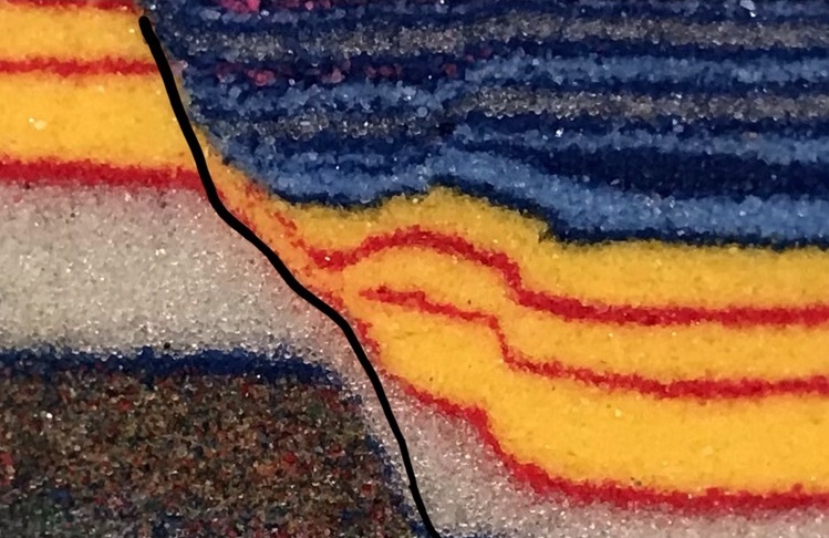
The model of extensional deformation shown here contains an unusual (?) detail that results from initial folding of the yellow and red layers before they were cut by faults. The model is dominated by normal faults, as one would expect from extensional deformation, but it also contains two minor reverse faults despite only experiencing extensional movement. The reverse faults show a tiny amount of displacement, but they are clearly visible as layer offsets at each end of the yellow and red layer zone in the graben (downthrown block).
The reverse faults are indicated by black lines in the image below; the black arrows indicate relative movement.
These minor reverse faults appear to result from fault propagation folding that occurred at the beginning of the deformation sequence. Tightening of the syncline (U-shaped fold) that forms as the model started to move caused localized compression in the inner hinges of the fold (see sketch below). The surface effects of the reverse faults can be seen in the moving GIF; the yellow arrow points to where the most obvious surface expression ended up once it dropped further into the basin and was buried (the GIF only shows the very beginning of the model run; it undergoes much more extension to make the final geometry shown in cross section). I don’t think that the reverse faults result from interaction of the yellow/red layers with the deep gray layer, as none of the basin fill layers show reverse fault disruption.

The line drawing below offers a general conceptual representation of where compression (squeezing) developed in the hinges of the fold. This compressional stress produced the small reverse faults; they are most definitely limited to these very loczalized zones in the model. Stretching indicated on the crests of the outer fold hinges causes cracking visible in the GIF above. The line drawing below only focuses on the yellow/red layer zone, which responded to initial normal faulting below it in the deep gray layers. The deep gray layers are intended to represent metamorphic or intrusive igneous “basement” rock.
Compression in the inner fold hinges is magnified by the thickness of the yellow sequence, which is a very strong, brittle sand, and the presence of the weak white microbead layer beneath it. The microbead layer allows the yellow layer to initially fold when the model starts moving. Without the microbead layer, faults would cut through all layers at the onset of movement. In the layer sequence used here, the weak microbead layer disconnects the deep strong layer from the yellow/red layers, allowing the initial fold to develop before faulting ultimately breaks through to the surface.
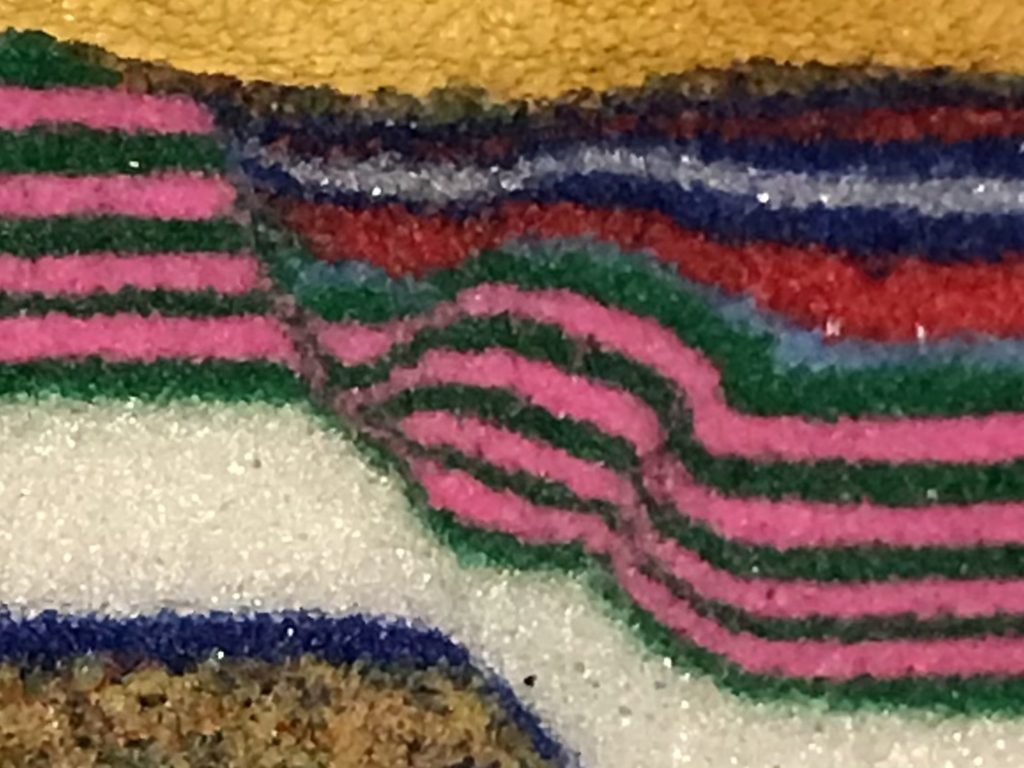
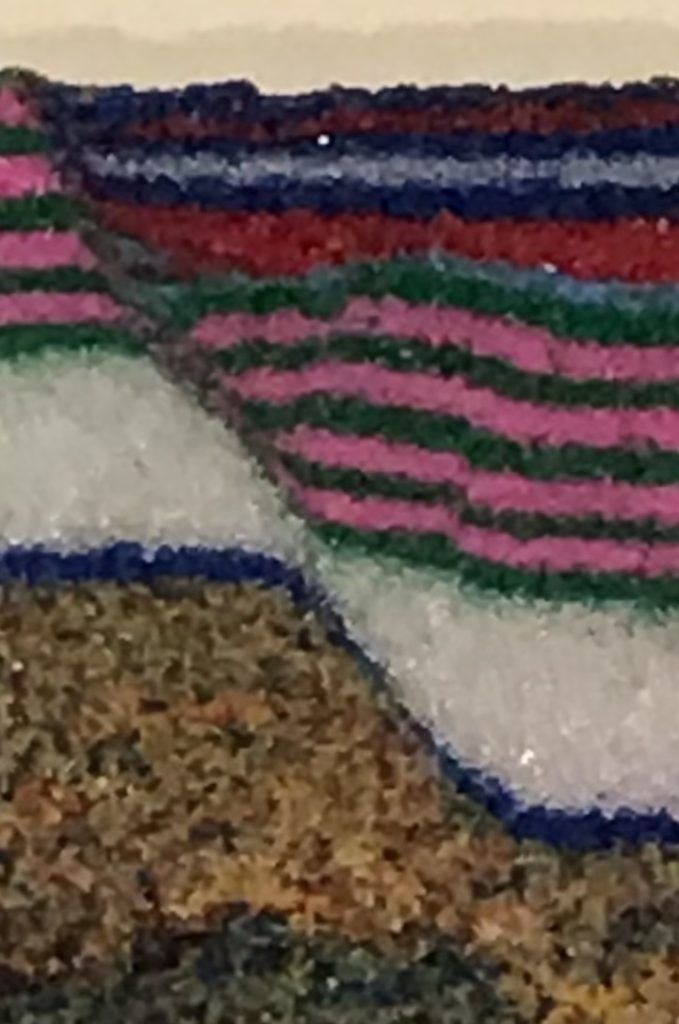
The different mechanical properties of the layers are apparent in the dip angles of the normal faults in the model. The master fault on the left side of the model (black line) is less steep in the weak microbeads, an expression of how their failure behavior differs from the stronger layers above and below. The anticline (convex-up fold) in the yellow sequence at the center of the image is a result of the shallowing of the master fault (more on this in another post).
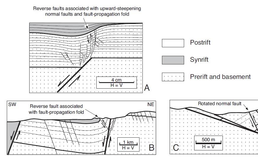
Simple models like this one are difficult to specifically scale to particular tectonic examples, but the basic geometric relationships that develop in the model do have documented analogs. The images below are from Figure 10 of Withjack et al. (2002), available at this link. It shows similar small reverse faults in a clay cake model (A) and a real-world example from the Suez Rift Basin (B).