by Philip S. Prince

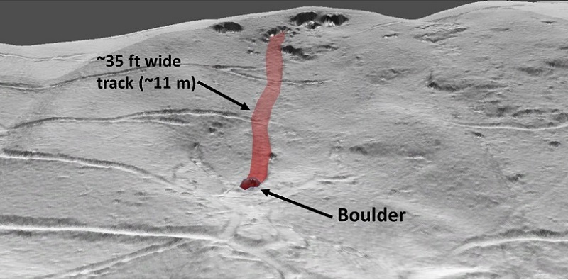
A few weeks ago, after years of “lidar surfing,” I finally encountered an Appalachian boulder that left clear evidence of its sliding path down a mountainside. Large boulders are common throughout all of topographically rugged Appalachia, but they typically reveal little or no evidence about their paths from upslope sources to their current resting places. This Macon County, North Carolina, boulder is a rare exception, as it carved a distinct groove or track on the land surface that can be followed from cliffs upslope to the boulder’s current position.

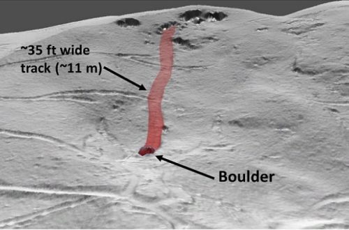
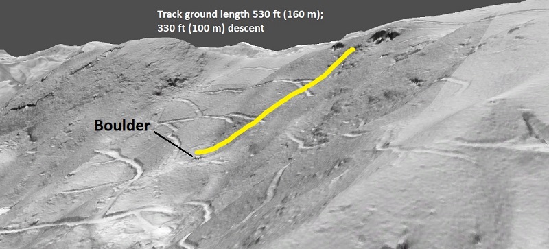
The boulder is about 10 meters (33 ft) wide at its widest. Its thickness is unknown, but it is likely several meters thick, and is sufficiently large to “stick up” in the 3-D Arc Pro GIF below.

Like so many Appalachian slope failures, the age of this “boulder slide” is unknown. Logging roads that are likely several decades old cut across the track, and no disruption to trees is apparent in aerial photography, so the event is presumably at least ~100 years old. Given the lack of similar tracks on other boulders in the region, these features clearly don’t last forever. This one is likely “young” in the overall context of processes that alter visible details of the ground surface and soil profile in this humid-temperate region.

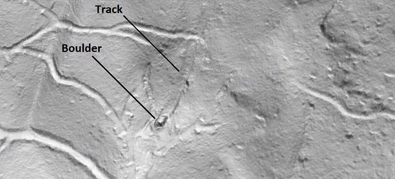
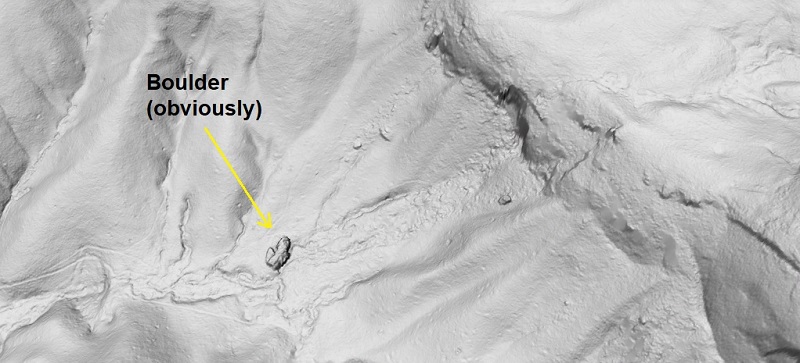
A particularly interesting detail of the boulder and its trip downslope is the pile of “plowed” soil visible at the boulder’s leading edge. The lidar signature of the soil pile suggests it is at least 1 meter (3.3 ft) high.

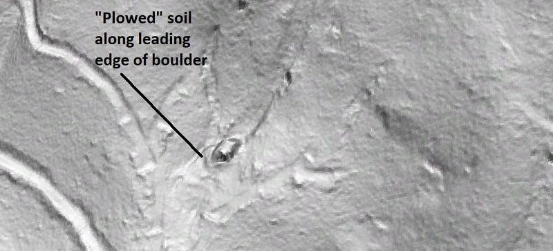
The “plow-pile” at the tip of the boulder remains visible even in a very close zoom. Several graded areas are visible near the boulder; they presumably relate to logging operations. Fortunately, they stayed far enough away to avoid disturbing the plow-pile.

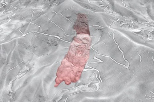
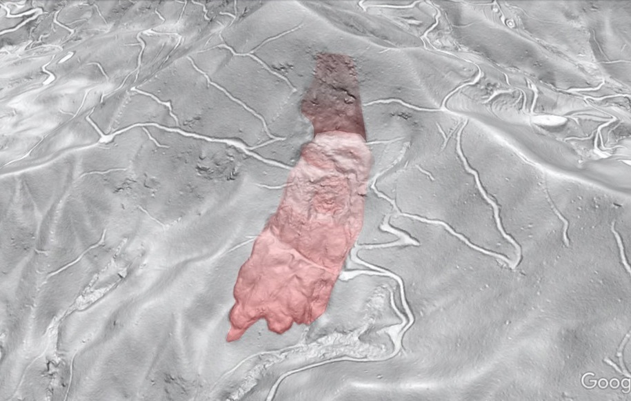
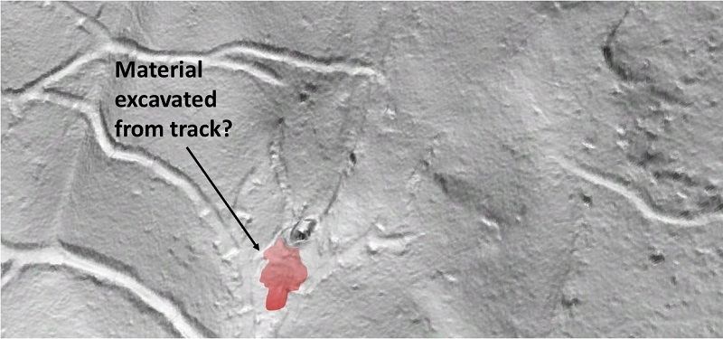
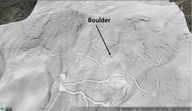
The length and width of the track indicate that a large amount of material was pushed out of the way by the sliding boulder. Some of it is visible piled along the edges of the track, but additional material was likely driven ahead of the sliding boulder, which may have moved during very wet conditions. Lidar suggests significant excavated material may be present just downslope of the boulder, but field verification of this idea is needed. The red polygon in the image below suggests where this excavated soil may have been deposited. This image also shows the track nicely.

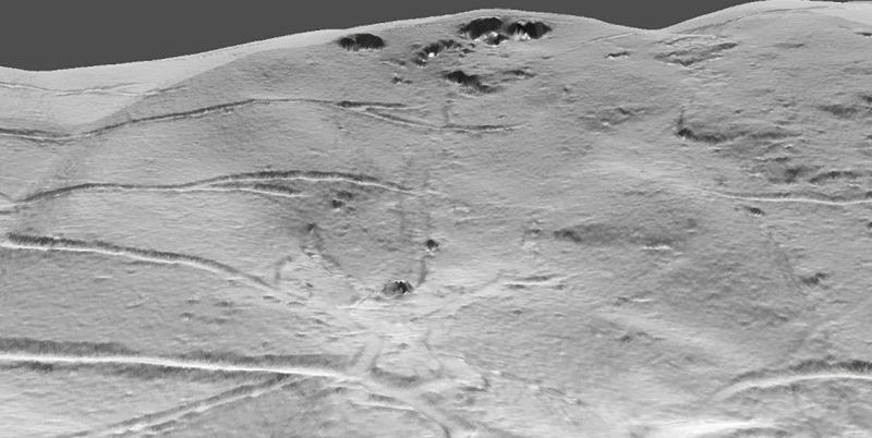
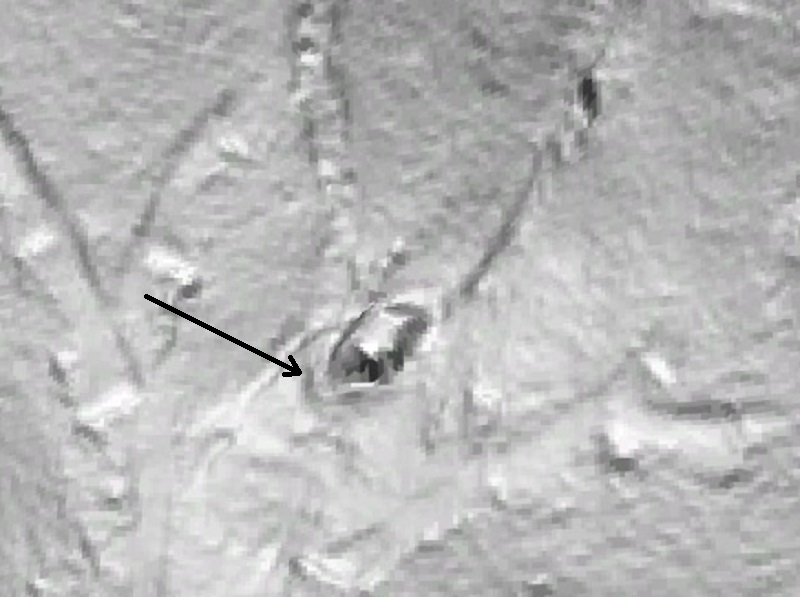
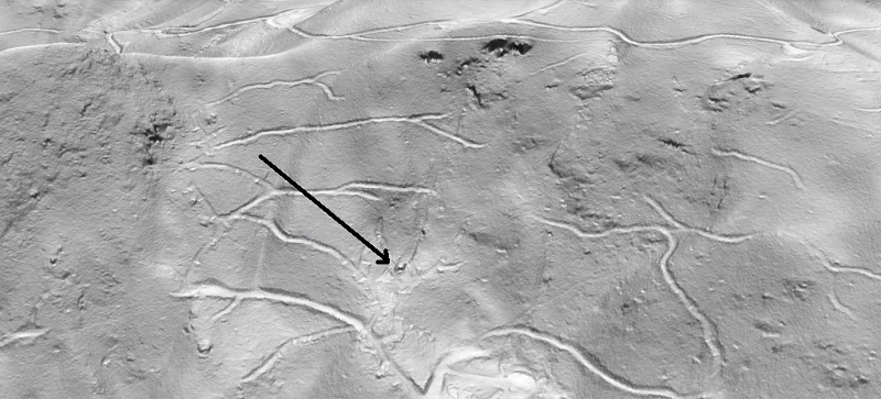
While the boulder would be very impressive in person, it is a tiny feature on the mountainside as a whole. The boulder initially caught my attention due to its bold outline, and the track only became noticeable after zooming in. The black arrow in the first image below points out the boulder. The track is faintly visible once you know it’s there, but it isn’t exactly eye-catching. The second image is from a slightly different vantage point in a kmz file, and the boulder isn’t labeled (do you see it?). On some screens, I think the boulder and track look better in the first ArcPro image; on others, I find it more visible in the kmz.

The boulder descended about 100 m (330 ft) in 160 m (530 ft) of ground-length travel. Based on the appearance of the track, I presume it slid the whole way, and probably detached from a downslope-dipping outcrop to start its journey in a favorable orientation.

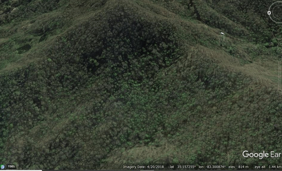
In addition to just being interesting to look at, this boulder and its journey are worth considering from the standpoint of human-landscape interaction. People live on these slopes, and the GIF below shows that a house is situated directly downslope from the boulder. The boulder came to rest where the steepness of the slope locally decreases, and its sliding style of travel probably caused it to stop as soon as the necessary steepness was lost. A tumbling and bouncing boulder probably would traveled farther, and a few noticeable boulders are certainly downslope of the house, though none of them show any indication of how they got there. Understanding how details of topography, along with movement style (tumbling vs. sliding), can alter the downslope travel of large rocks is worthwhile information in inhabited mountainous areas. Lidar imagery is critical to learning more about these processes.

So, are there other examples of this? I have written about a few other lidar features that suggest details of boulder and rockfall travel, and I have seen one small boulder in the field which had recently rolled into place and left interesting marks in the soil and on trees upslope. While boulders are everywhere in the rugged portions of Appalachia, traces of their movement appear to be eliminated by erosion and vegetation cycles MUCH more quickly than the boulders themselves weather away. Plenty of additional examples surely exist, but the intensity of lidar inspection necessary to find them would likely cause blindness or some other negative side effect, so I don’t plan to begin a boulder track search anytime soon. The only other boulder I know of that might show a track is in Transylvania County, North Carolilna, near Johns Rock. It is massively huge–about 40 m (132 ft) long, and probably 15 m (~50 ft) thick–and it surely slid from the obvious dark scar on the cliff line up and right of its present resting place.

The land surface is rough and irregular between the boulder and its source, which might suggest lasting disturbance from the initial failure and sliding event. This texture could result from water erosion and accumulation of smaller rock fragments from the scar. Like the Macon County example, the entire area is thickly re-vegetated. Field work might help sort things out, but, as in so many other cases, high-resolution lidar imagery might be the best source of information.

by Philip S. Prince

In addition to the Split Mountain slide described in the previous post, Thomas L. Clingman referenced other slope failures known to have occurred in the western North Carolina Blue Ridge during the early to mid-19th century. Geographical descriptions of the slides’ locations vary in quality, but one feature initially reported by Silas McDowell of Macon County proved easy to locate with the aid of lidar-derived slope-shade (an inverted black and white slope raster) imagery. Like the Split Mountain slide, the Macon County feature is entirely re-vegetated and not noticeable without high-resolution, lidar-derived imagery. The slide is shown in the GIF below, and the Google Maps image that follows shows the feature’s location with respect to Franklin, North Carolina.

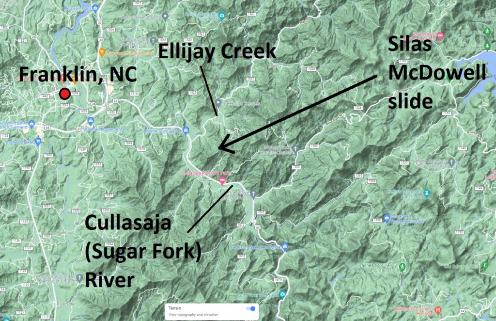
This slide was described as being located on the north slope of the ridge separating Ellijay Creek from the Sugar Fork River (today’s Cullasaja River), and this simple description was adequate to find the feature due to its size, displacement, and surface texture. McDowell described the slide as a “violent shock” which opened a “chasm” that remained visible for many years after the initial event. The date of the slide is unknown, but probably occurred around the 1850s.

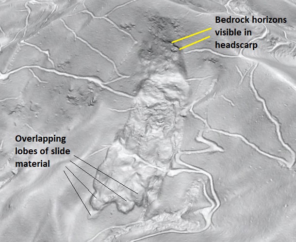
The slide shows a dramatic and steep headscarp, which cuts bedrock horizons. I am unsure of the bedrock lithology, but broad-scale mapping in the area suggests it is likely biotite gneiss. The texture of the slide mass and the lack of an intact slide block is consistent with rapid emplacement with a minor component of flow. The extent of the rupture surface is unclear, but the overlapping lobes of material at the slide toe are probably well downslope of the base of the rupture itself.

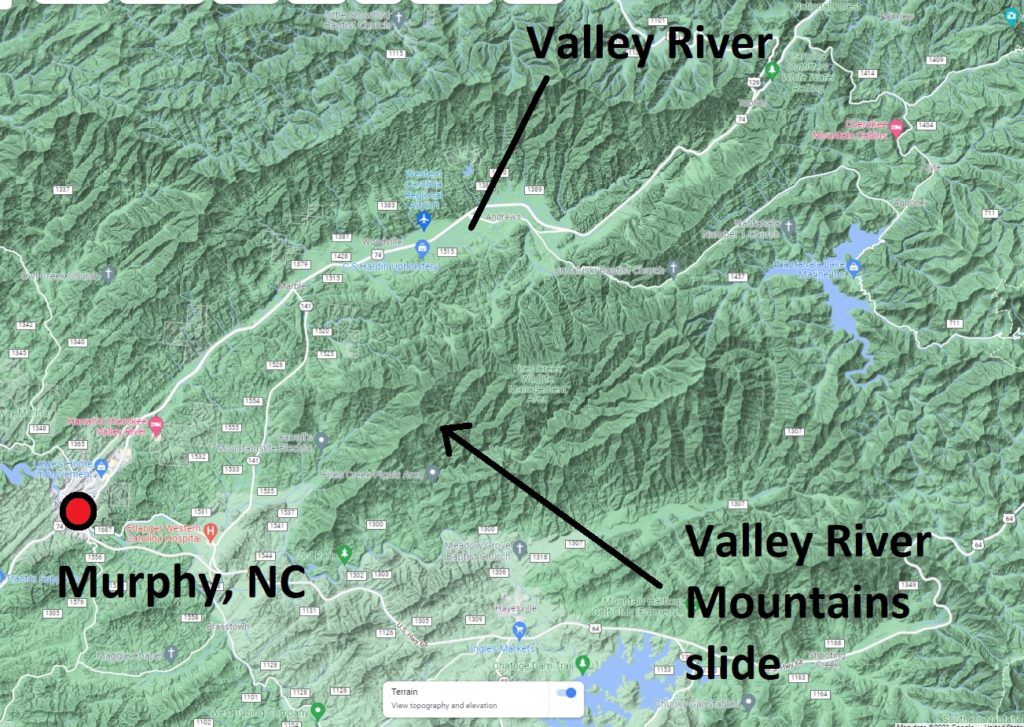
The use of the word “shock” in the description of the Macon County slide shows it refers to the slide event itself and not to seismicity that caused the failure. The preceding slide description in Clingman’s writing supports this idea, as an 1829 slope failure in the Valley River Mountains in Cherokee County is said to have followed an earthquake, which is described as “a shaking of the ground.” I searched for this slide, but I was unable to find anything as obvious or dramatic as the Split Mountain and Silas McDowell features. The only plausible candidate, which is actually located just inside Clay County, is shown below. The Google Maps image shows its location within the Valley River range east-northeast of Murphy, North Carolina.

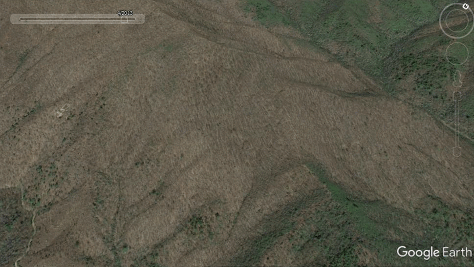
The description of the Valley River Mountains slide as “partially filled in” suggests it was less dramatic in appearance even in Clingman’s day, so perhaps the somewhat muted feature visible today with lidar is indeed the slide in question. Lateral scarps are faintly visible, and more recent activity at the toe of the slide might be evidence of reasonably young age. A presumably older slide is visible to the lower left of the slide mass outlined in the GIF. The appearance and size of this slide suggest it has probably experienced ongoing, episodic movement, so the 1829 failure may have only represented localized movement of a portion of the overall feature.

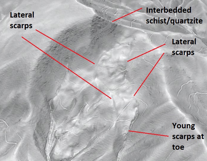
Bedrock horizons (schists and quartzites) visible on the peak above the slide indicate its dip slope context. The extent to which bedrock is involved in the slide (as opposed to overlying colluvium and soil) is unclear. Several other dip slope slides occur in the immediate area, but all appear significantly older.

In addition to providing interesting information on these slope movements, Clingman’s “Volcanic Action in North Carolina” manuscript provides a fascinating look into prevailing ideas about Earth process in the mid to late 19th century. Kathy Ross kindly provided the link to the entire manuscript (click here), which is a quick and worthwhile read.

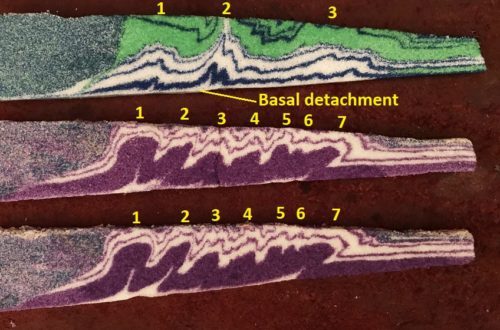
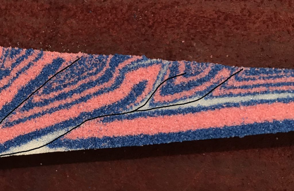
These fold-thrust belt analog models contain anticlines with interesting changes in structural style from top to bottom. Anticlines are labeled by number, and all are associated in some way with faulting originating from the basal detachment of the models (which is only labeled on the top model).

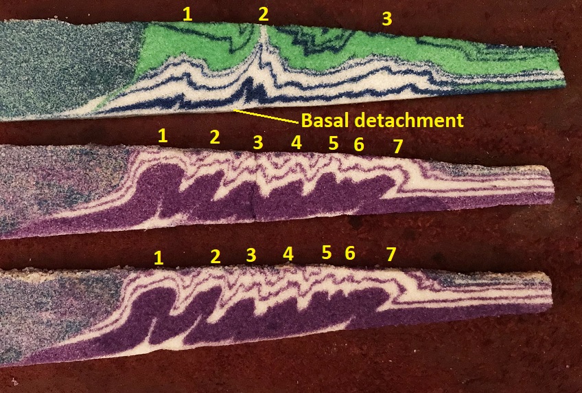
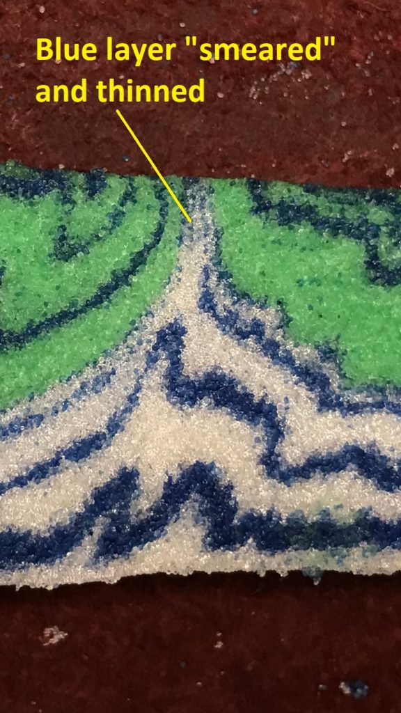
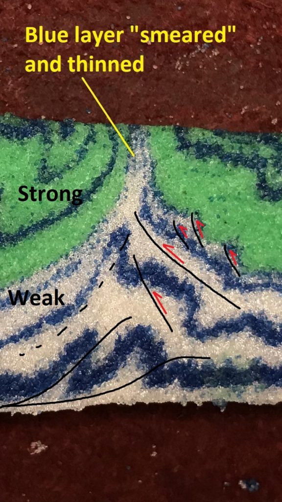
Anticline 2 in the top model is extremely narrow at the model’s surface, with vertical limbs that quickly transition to lower dips in adjacent synclines. A thin, vertically extensive “smear” of the upper two white layers has been squeezed into the core of the anticline. The blue marker layers have been stretched and thinned in the squeezed area until they are almost not visible.

Deeper layers show more typical thrust imbrication and shortening/thickening expected from compressional deformation. Some of the smaller folds deeper in the model have developed steep limbs on their hinterland side, suggesting minor backthrust movement.

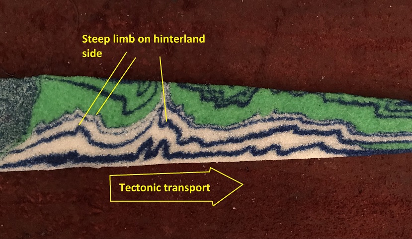
Backthrust movement (shown by red arrows below) within the white layers is also implied by the overall shape of the anticline and the fact that the deeper thrusts do not propagate upward through the entire section.

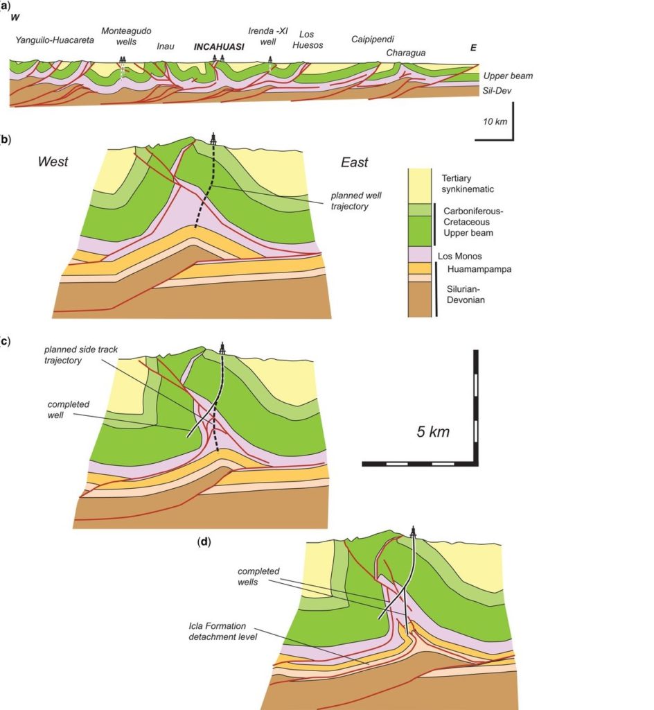
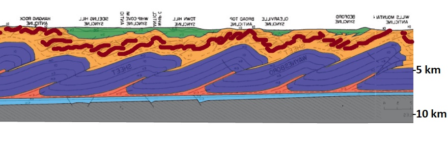
Similar structural styles are commonly interpreted in the Bolivian and northwest Argentinian sub-Andes, where stronger upper layers lift off of deeper layers along weak shale horizons (lavender, between green and brown, in the sections below). In the model, the green and blue layers are stronger than the white layers, whose weakness allows the green layers to be squeezed together in the tight anticline. The schematic below from Butler et al. (2019) shows interpreted (b) and drilling-confirmed (d) geometries of the kilometer-scale Incahuasi anticline of Bolivia.

The purple models use stronger layers (solid purple) at depth, with weaker glass microbeads (white) with thin purple marker beds higher in the section. In this case, anticlines are more complex near the surface of the model, with a simpler structural style within the thick purple horizon at depth.

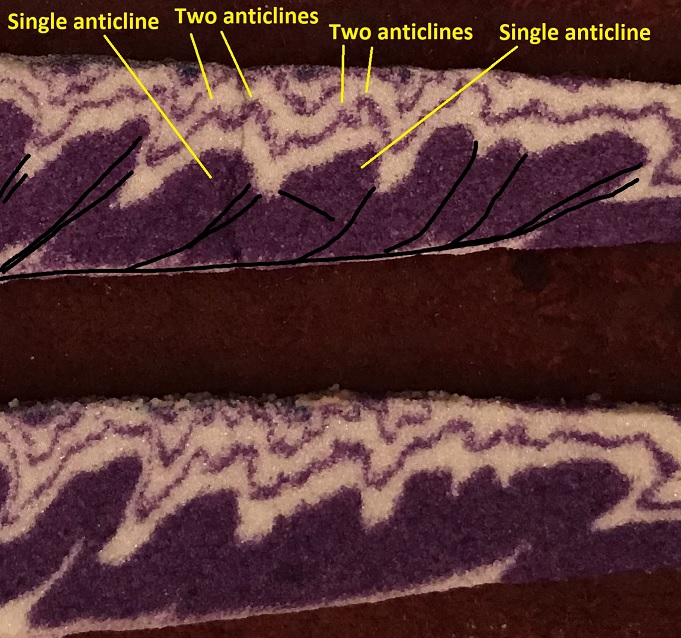
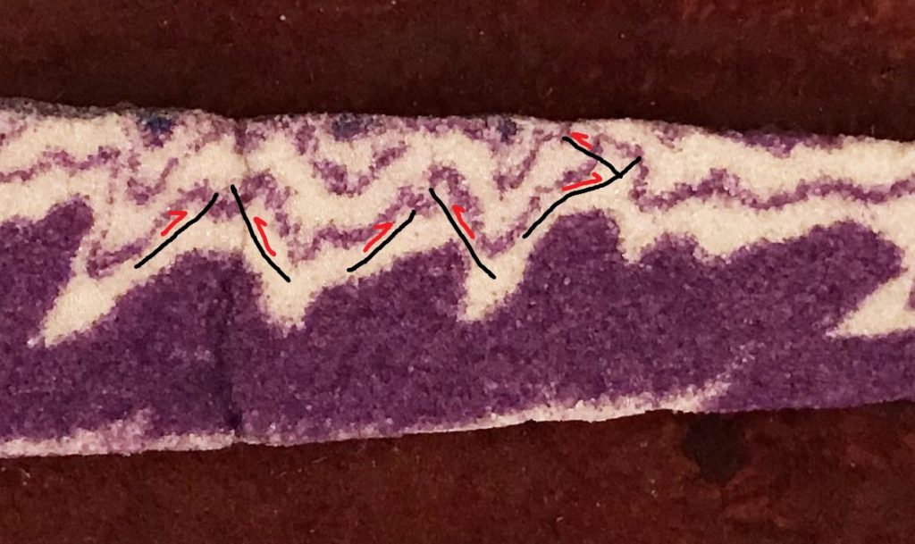
Many of the anticlines, which are fundamentally thrust fault-controlled (black lines in the image above), develop two or more small folds atop the a single fold crest in the deep purple layer. These small folds occasionally have steep limbs on their hinterland side, consistent with backthrusting.

The small-scale folds are clearly part of overall anticlinal structures affecting the whole section, but they could present challenges in interpreting the comparative simplicity of the deeper structure. Central Appalachian Valley and Ridge structural style (a common reference in these posts) from Kulander and Dean (1986) is a good example of complex surface structure above comparatively simple and regular deep structure. Below, the tightly buckled and faulted dark red layers generally follows the waveform of the deeper structure, but hosts several small anticlines and synclines above a single deeper anticline.

The complex structures in the three models above develop due to the strongly contrasting layer strengths in the models’ layer packs. Fold-thrust analog models using a more mechanically-consistent layer pack produce simpler anticlines above thrust splays rising from the basal detachment. In the example below, the pink and blue layers are mechanically the same, while the white layers provide detachment horizons.

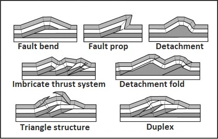
Because rock sequences (either sedimentary or otherwise) experiencing tectonic deformation are likely to contain mechanically-differing horizons, complexity in fault-related fold structures is common. Analog models can reproduce some of this complexity, and structures made from mechanically-contrasting materials can contain combinations of the main fault-related fold styles (below) within a single structure. The classic image below, sourced at this link, is from Roder (2012) and is drawn after Mitra (1992).

An important take-away from the images above and verified geometries in real anticlines (as well as models!) is that interpreting the subsurface by projecting surface orientations downward must be done with structural style in mind. Surface data is certainly critical to geologists’ efforts to understand deeper structure, but different styles of movement and thus different angular relationships that operate at various depths can lead to confusion and bad results. In many settings, accurate subsurface interpretation is nearly impossible without seismic imaging or drilling records.

Identifying and visualizing fold structures is a major part of any geology student’s experience, with most students’ first encounters with anticlines and synclines involving images like the ones below, used by the US National Park Service.

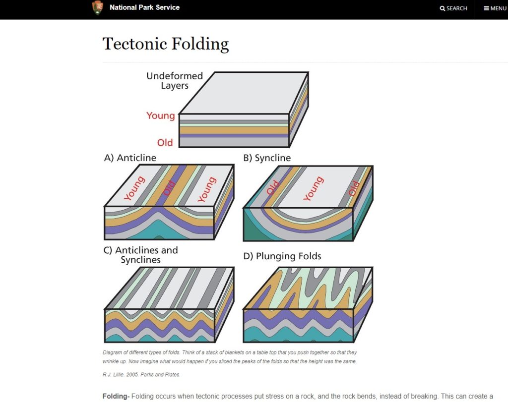
These simple representations are a necessary starting point, but they do not associate the folding with movement or the characteristics of the material responding to the movement. Real-world structures reflect a combination of kinematics and materials and the complex interplay between the two. Learning to understand the more nuanced aspects of rock deformation is a key part of advanced geologic study and critical to producing accurate sub-surface interpretation.