-
Lidar-derived imagery of 1949 debris flows on North Fork Mountain, Grant County, West Virginia
by Philip S. Prince
An intense convective storm on June 17-18, 1949, produced approximately 16 inches (400 mm) of rainfall in southern Grant County, West Virginia. The intense precipitation caused numerous debris flows on North Fork Mountain, a ridge developed on moderately dipping Siluro-Devonian sandstones on the back limb of the Wills Mountain anticline.
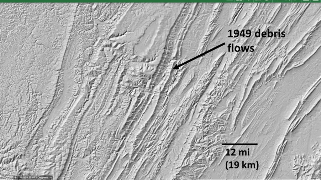
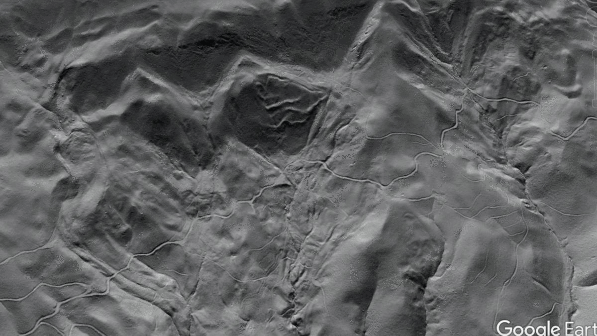
Cenderelli and Kite (1998) mapped some of the flows in detail (along with others immediately southwest resulting from a 1985 storm), and the resulting paper is a great read. Features related to the flows are very visible and distinct in lidar-derived hillshade and slope-shade imagery. I produced several .kmz overlays of the area for a 3-D view, and the outstanding West Virginia Landslide Tool offers streaming plan-view surface imagery of the area. The results of the flows are locally visible in aerial photography, particularly once their position is noted using lidar functions. All measurements in the following images represent distance over the land surface.
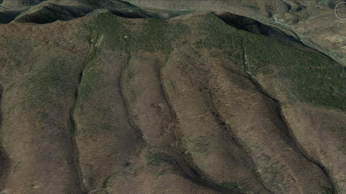
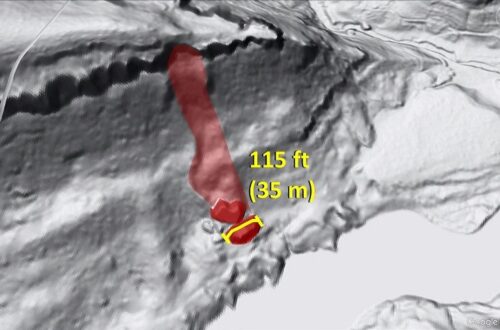
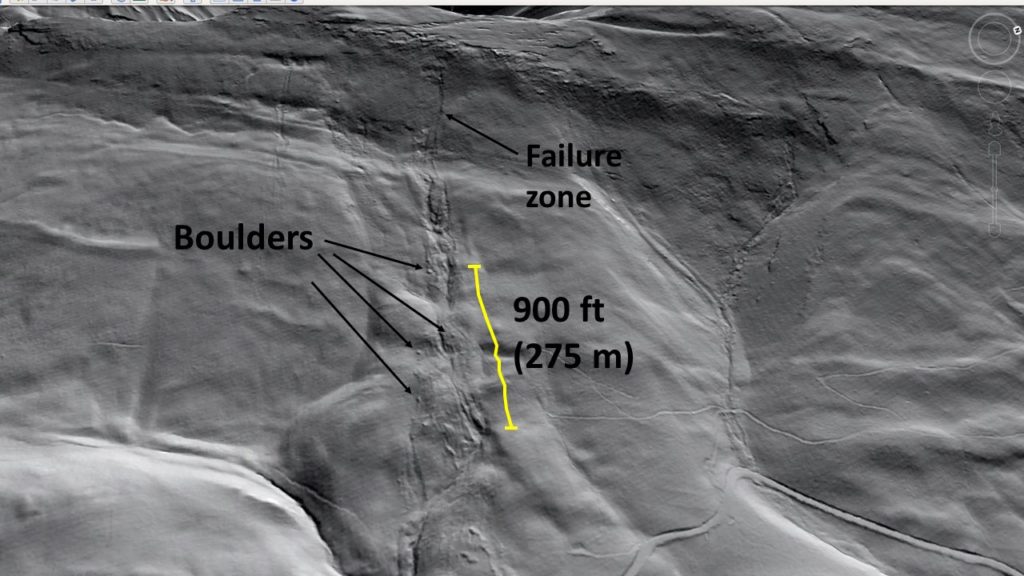
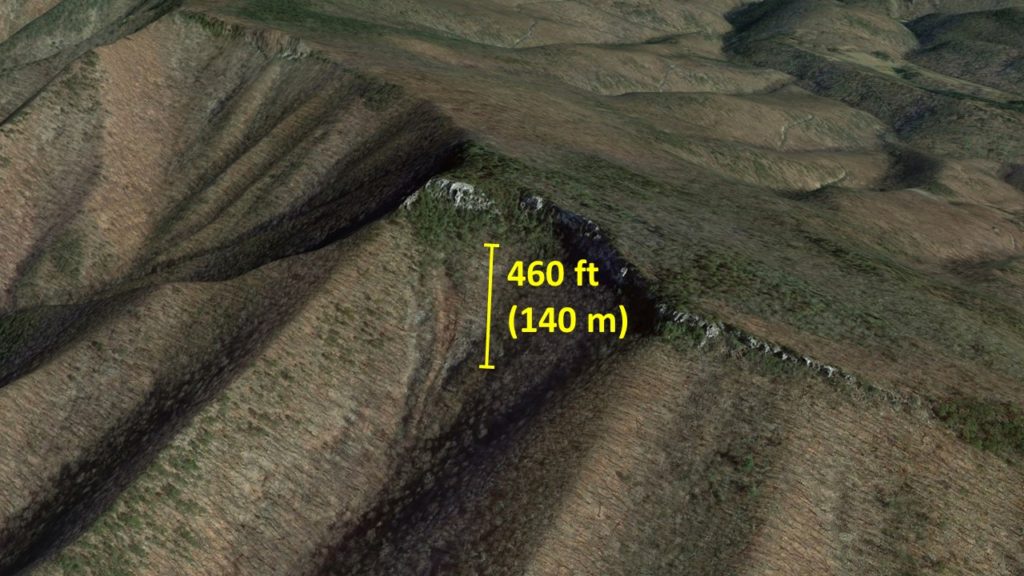
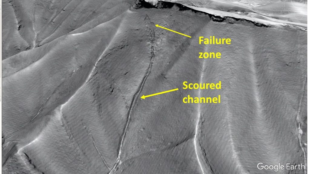
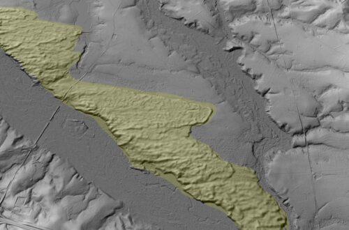
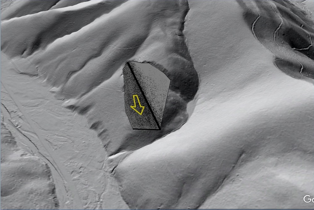
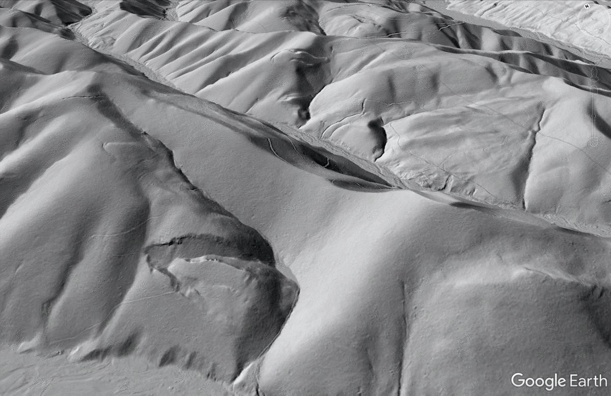
The GIF above shows the southeast slope of North Fork Mountain, which is a dip slope developed on the resistant Siluro-Devonian sandstones. Failure zones where the flows initiated are visible as white patches where the sandstone was laid bare by failure of overlying soil, colluvium, and regolith. The flows scoured the channels for a considerable distance downslope, and the effects of the scouring are also faintly visible in the aerial photography. The yellow polygon outlines an interesting translational landslide that presumably also occurred during the 1949 event. Numerous older slides are visible to its right. The GIF is centered on 38.967702N 79.249423W.
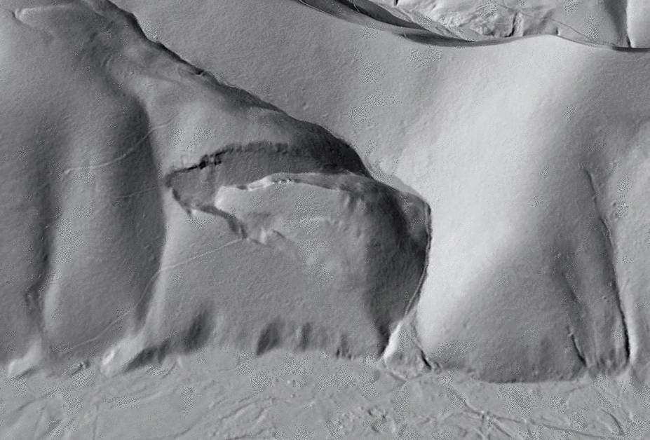
The debris flow feature at far right in the GIF above has a particularly interesting-looking failure (initiation) zone.
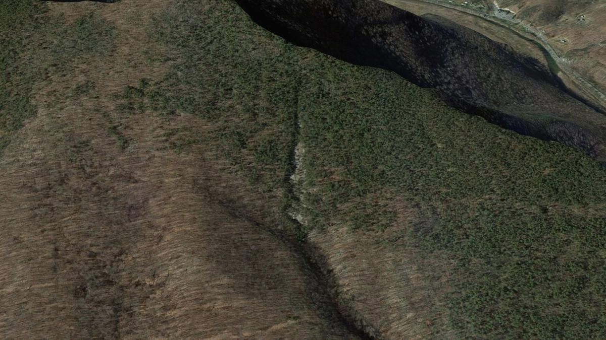
The elongated scar visible in the hillshade imagery coincides with exposed white sandstone bedrock. The scar widens downslope, which is atypical with respect to the other failure zones on the southeast side of the mountain.
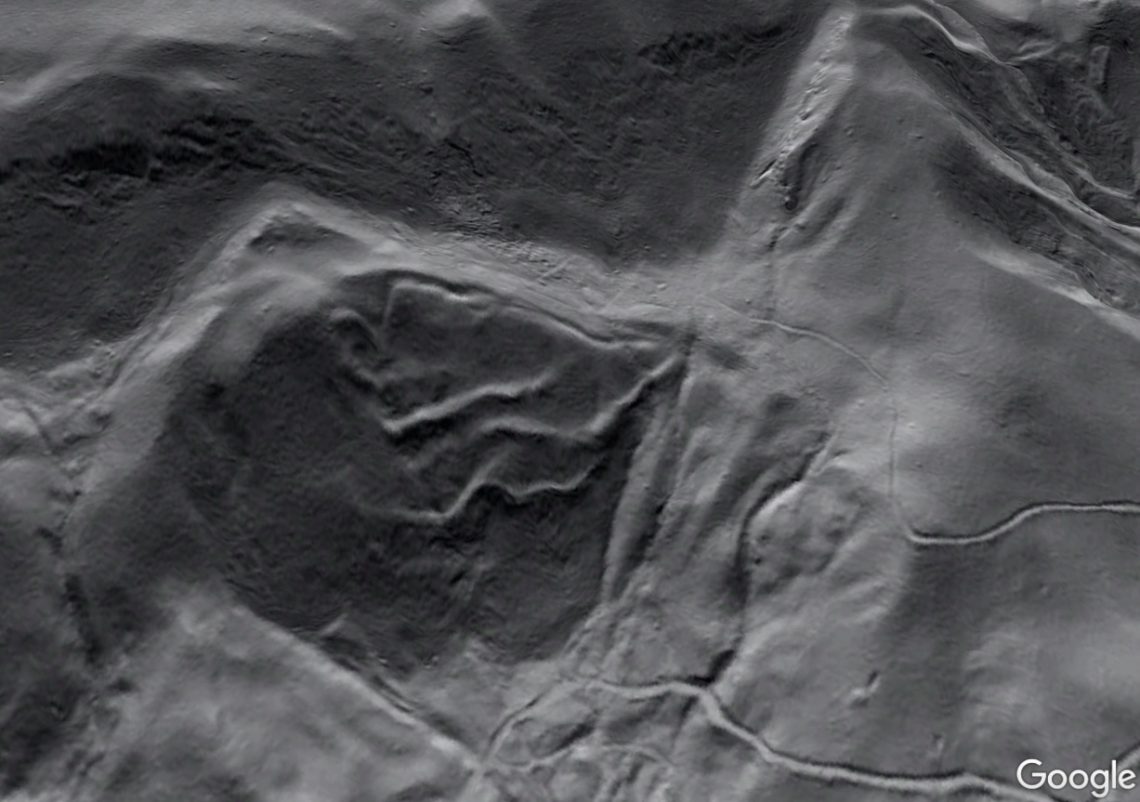
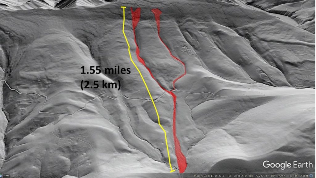
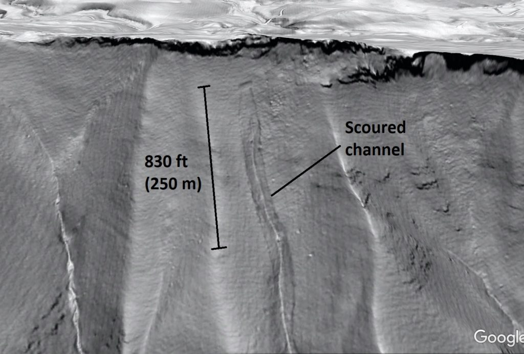
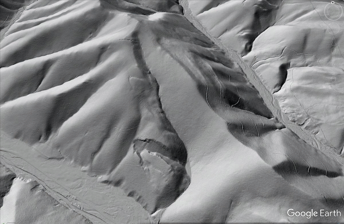
The longest debris flow features in this area extend about 1.6 miles (2.5 km) from failure zone to the downslope terminus of deposited material. The Austin Run flow, which is mapped in detail in Cenderelli and Kite (1998), is highlighted below. The flow with the elongated failure zone from the previous GIF traveled down the ravine at the right side of the image.
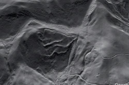
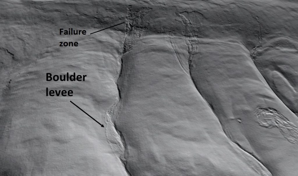
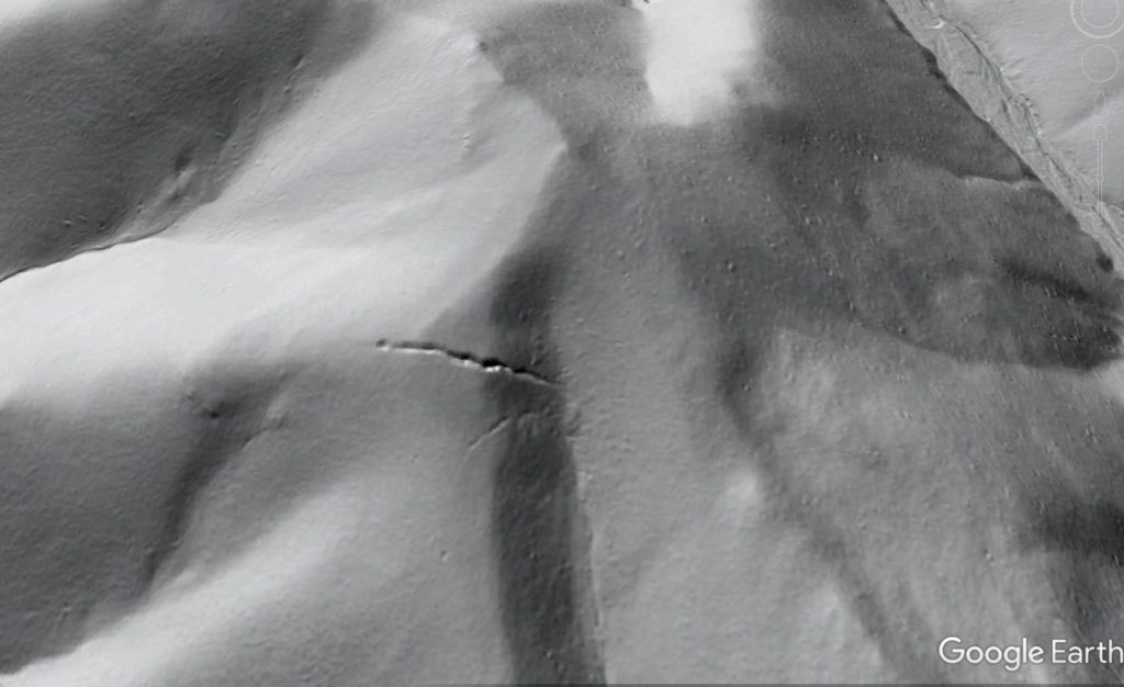
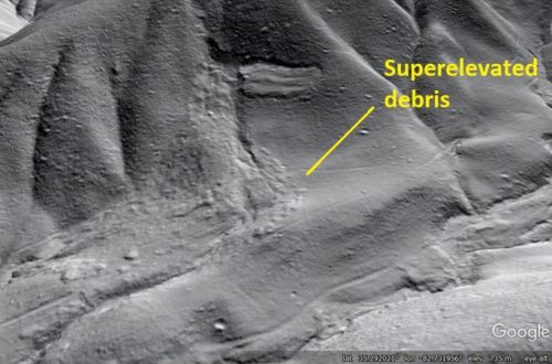
The hillshade imagery has adequate resolution to reveal small-scale features created by the flows, such as boulder levees deposited along the flow tracks. The boulder levees shown below are located just up and right of the “s” in “miles” in the image above. They provide some sense of the extent of the flow within the Austin Run stream valley.
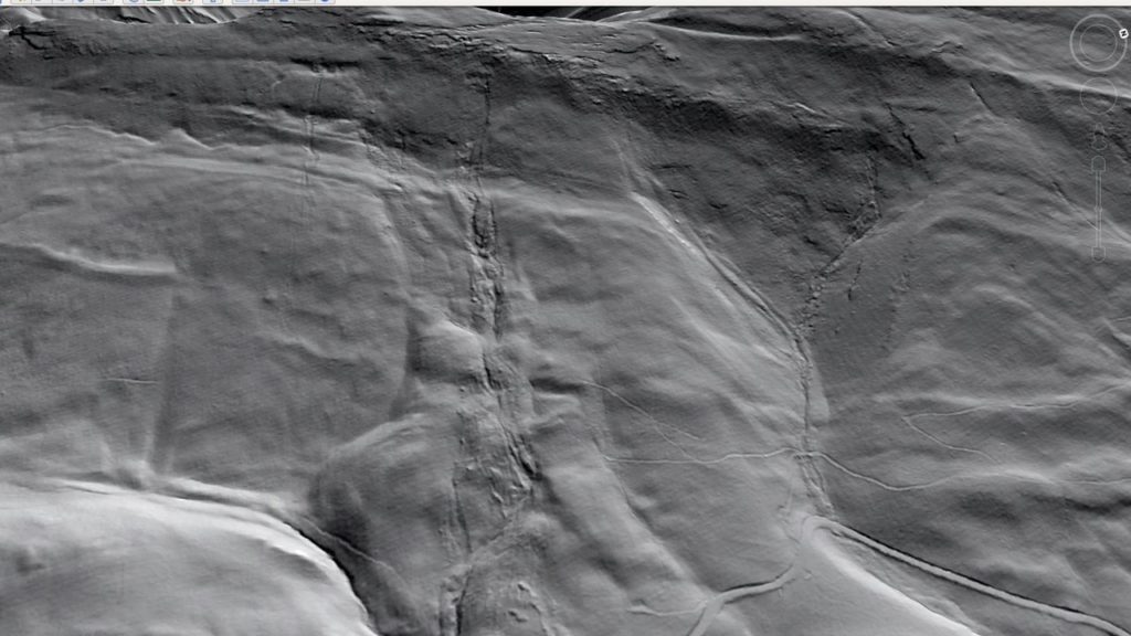
Boulder transport is also apparent in a significant flow to the southwest, which followed a less channelized path downslope. The second image below with no annotation shows how flow-related surface features stand out within the smoother surrounding land surface.
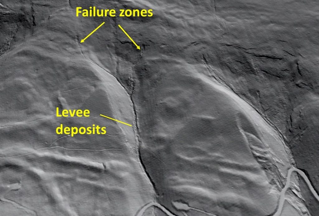
Boulder levees are also visible on a smaller flow track to the northeast. An interesting rock slide with a flow component at its downslope end is visible at lower right in the image.
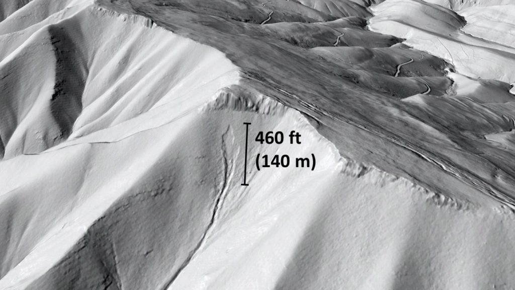
Considerable debris flow activity occurred on the northwest scarp slope of the ridge. The image below shows a well-defined failure zone just below the Silurian sandstone cliffs on the ridge crest.
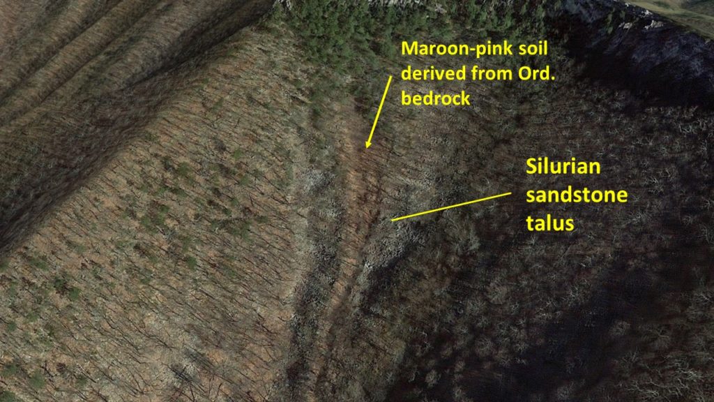
The northwest flank of the ridge is underlain by maroon sandstones of the upper Ordovician Juniata Formation just below the ridge crest. Martinsburg Formation shale is present beneath the Juniata, and the position of the contact is not immediately clear in the imagery. Much of the upper portion of the scarp slope is mantled by sandstone talus derived from the white Silurian sandstone cliffs at the ridge crest. The image below shows the same area as the previous image, with the sandstone cliffs, white talus, and failure zone scar visible.
The pink color of the failure zone scar is consistent with the Juniata (or potentially uppermost Martinsburg) Formation, and it contrasts sharply with the white sandstone talus through which it cuts. This flow may have resulted from failure of the talus pile at its contact with underlying residual soil or intact bedrock.
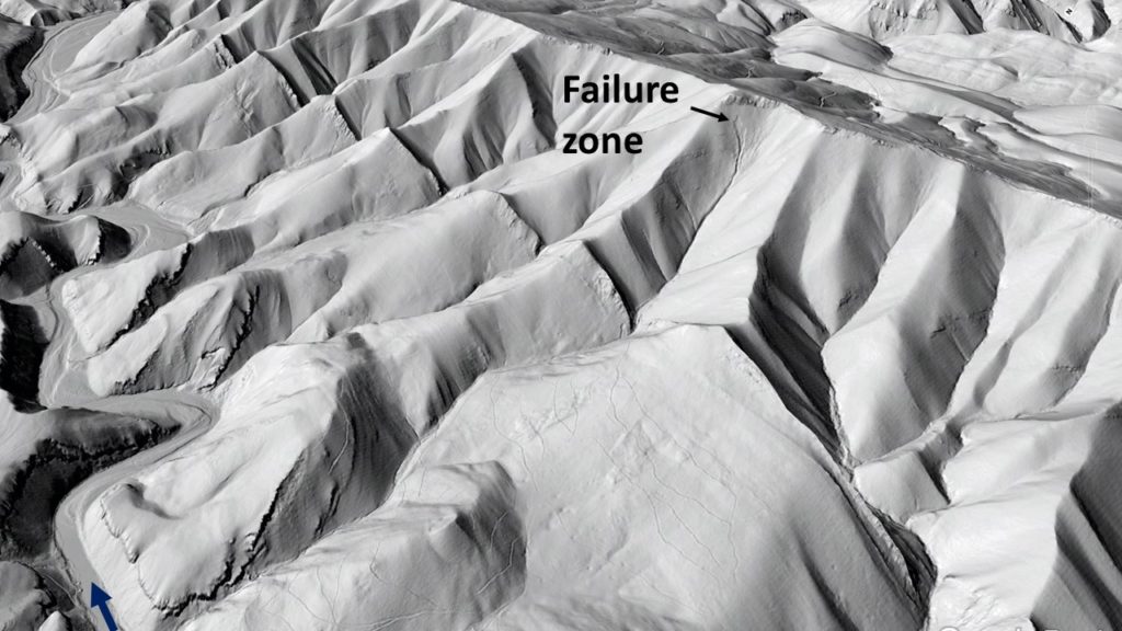
This flow, which is just north of the Kisamore Run flow described in Cenderelli and Kite (1998), appears to have traveled ~1.25 miles (2 km), essentially all the way to the North Branch of the Potomac River. The river channel and its flow direction are noted by the blue arrow in the lower left corner of the image below. The axis of the Wills Mountain Anticline is actually underneath the word “zone;” the apparent anticline just left of the center of the image is part of a complex structure that may involve passive backthrusts.
While I typically favor hillshade imagery for viewing slope failure features, slope-shade (inverted black-and-white slope raster) is necessary to appreciate the debris flow features on the northwest flank of North Fork Mountain. The GIF below shows numerous failure zones within the upper Ordovician interval. Failure zones have a different shape from those visible on the southeast, dip slope side of the mountain.
Slope-shade imagery reveals channel scouring related to the flow that left the pink failure scar.
Extensive scouring is also visible at the head of the Kisamore Run flow (see Cenderelli and Kite, 1998). This view gives some sense of the the amount of material entrained into these flows.
At the Potomac River gap at the north end of the mountain, slope-shade reveals a significant flow feature in an area completely shadowed in aerial photography.
Debris flow events present a significant hazard to life and property in all parts of the Appalachians. The 1949 event that created the features shown here caused 8 fatalities and displaced a tremendous number of residents. Detailed mapping of the type conducted by Cenderelli and Kite (1998) (as well as many other authors throughout the region), along with analysis of detailed surface imagery, can greatly enhance understanding of where debris flows begin and where they travel. This understanding, in turn, can potentially reduce the human impact of these particularly dynamic and mobile slope failure events.
-
Lidar hillshade imagery hints at the location of a future coal spoil landslide
by Philip S. Prince
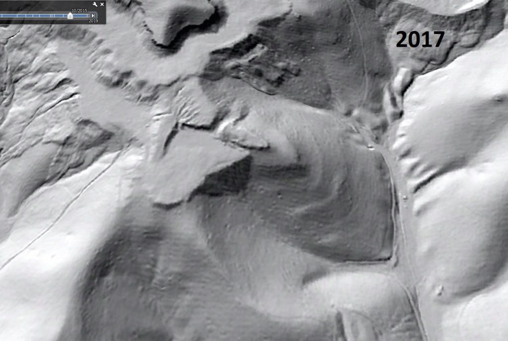
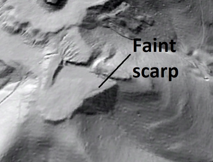
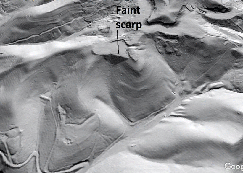
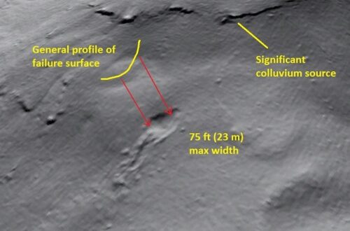
A coal spoil landslide in southeastern Wise County, Virginia, appears traceable to a faint scarp visible in the spoil pile in a 2017 lidar dataset. The slide pre-dates October 2019 Google Earth imagery and post-dates the 2017 lidar data acquisition. In the image below, the flat-topped spoil pile where the slide originated is readily visible near the center of the image. The “hairline” arcuate scarp is faintly visible at its edge; it is labeled in one frame of the GIF that follows, which also shows the slide (regional location and context are at the end of the post).
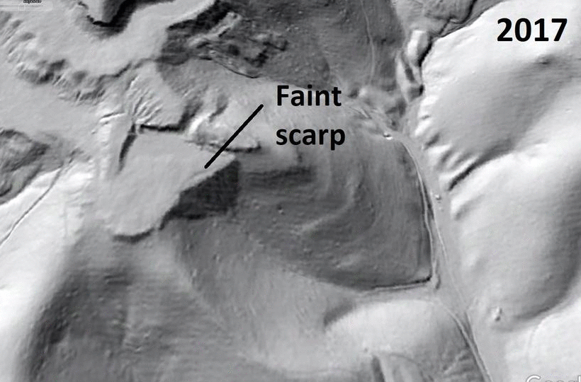
I first noticed the (very) faint scarp in 2018 while checking out lidar hillshade imagery of the Guest River Gorge to the west. Coal spoil landslides in the area turned out to be more eye-catching, which led me to look around for evidence of incipient failures. The flat top and ravine-fill location of the spoil that sourced the recent slide caught my attention, leading me to notice the scarp. Zooming in on the feature does not necessarily make it more visible, as it pushes the limits of resolution of the 1-meter lidar dataset.
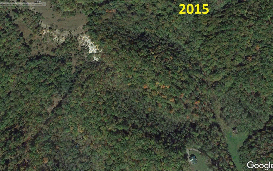
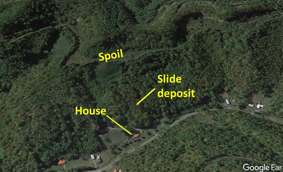
Today (Nov. 30, 2020), I decided to look at Google Earth imagery to check for any change at the location, and was not entirely surprised to see a slide had occurred at the scarp’s location. The GIF below shows 2015 imagery, the 2017 lidar overlay, and the October 2019 imagery showing the slide.
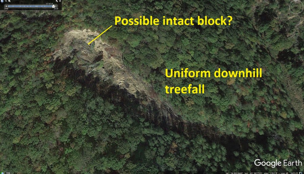
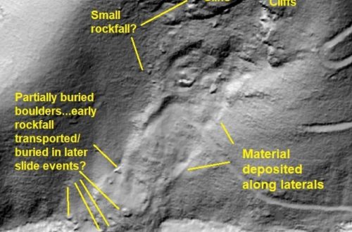
From its headscarp/initiation zone (IZ) to its downslope terminus, the slide extends over a ground length of ~830 ft (~250 m). The slide appears to have progressed to a flow and followed the ravine downslope, passing to the north of a house situated above the ravine. Several downed pine trees with green needles are visible near the headscarp/IZ, suggesting the slide probably occurred in 2019. Tree fall patterns indicate a partially intact block may be present near the head of the slide, with the downslope flow component knocking trees down in a uniformly downhill direction.
The perspective view below shows the path of the slide/flow down the ravine.
To the north of this location, another coal spoil slide is visible in close proximity to a house. I am unsure of the relative timing of the slide and house construction, and the vegetation suggests the slide is many years old but younger than the forest growth around it. The GIF below shows subtle distinctions in vegetation atop the slide and in the surrounding forest. While these coal spoil landslides are modest in physical scale, they are large enough to significantly impact home sites as well as roadways which may offer the only access to portions of this rugged landscape.
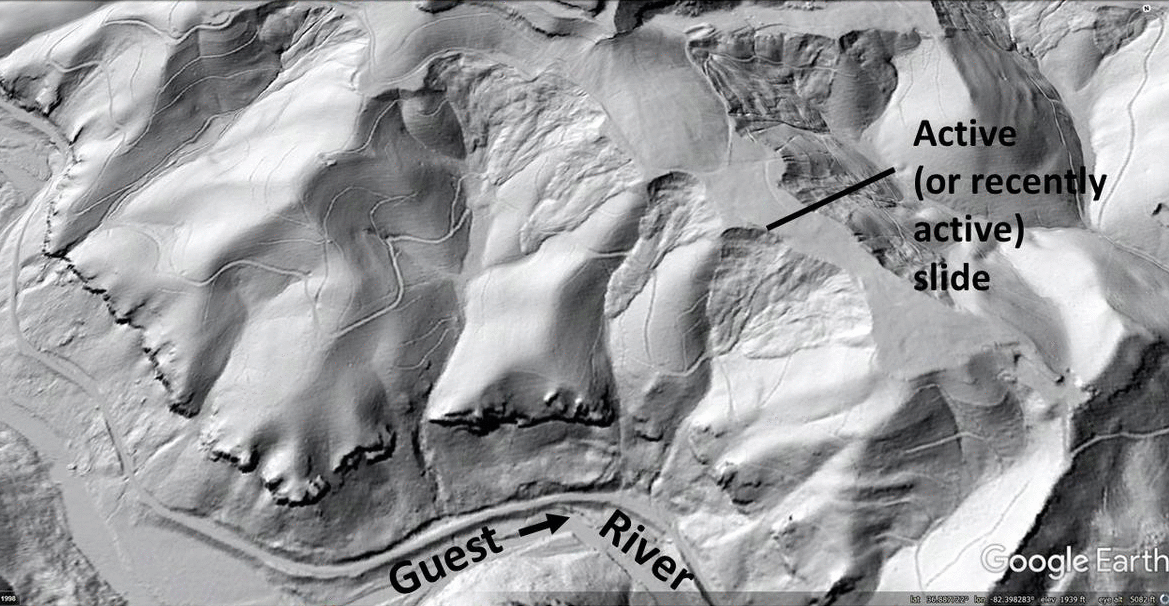
To the west along the Guest River, extensive failures are visible along spoil piles developed on a ridge crest. One failure is active or recently active, with sliding beginning between 2012 and 2015. Google Earth imagery suggests some movement may still be occurring, as bare earth is visible on a slide feature in the GIF below.
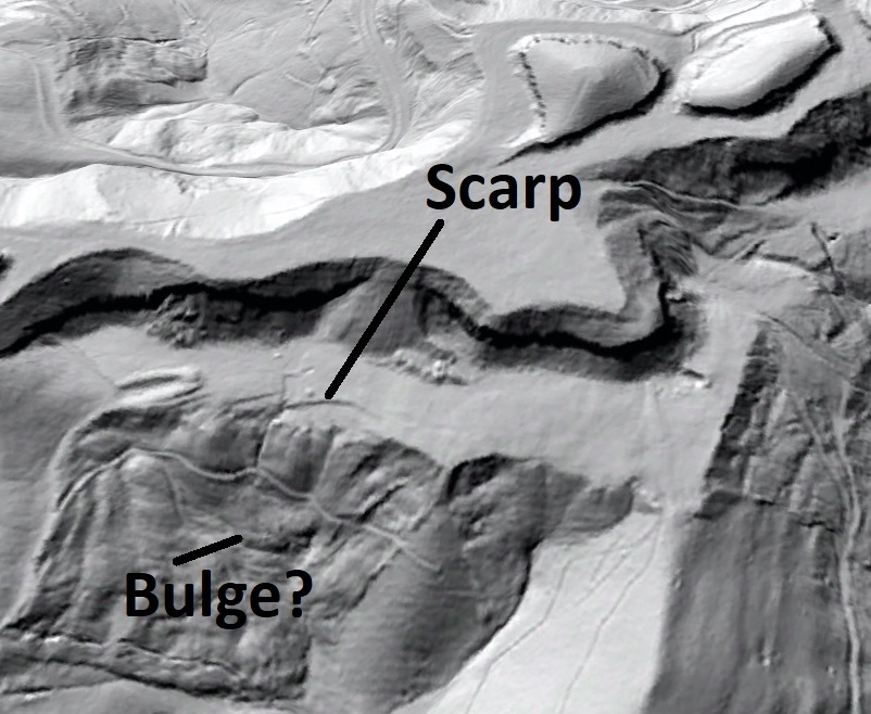
In addition to the scarp associated with the 2019(?) slide, a similar but larger scarp immediately to the west is more visible in lidar hillshade imagery but has yet to produce a failure.
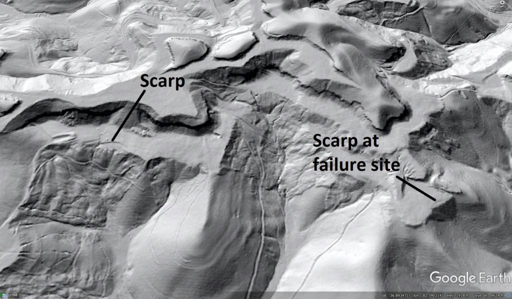
Closer inspection of this slightly larger scarp suggests the slope may be bulging below it, but this is speculative in the absence of field work. Fortunately, the ravine below this scarp is completely uninhabited.
The scarp-to-slide progression visible in the lidar and Google Earth imagery is an interesting example of how detailed lidar data and regularly updated land surface imagery can be used to understand landscape change over short timescales. Due to the extensive forest cover in the region (even in reclaimed mining areas), relevant features indicating imminent or ongoing ground movement can be nearly impossible to see from the air or even on the ground. Using lidar to “see through the trees” greatly enhances the ability of geologists and engineers to identify and address land stability issues in an efficient manner.
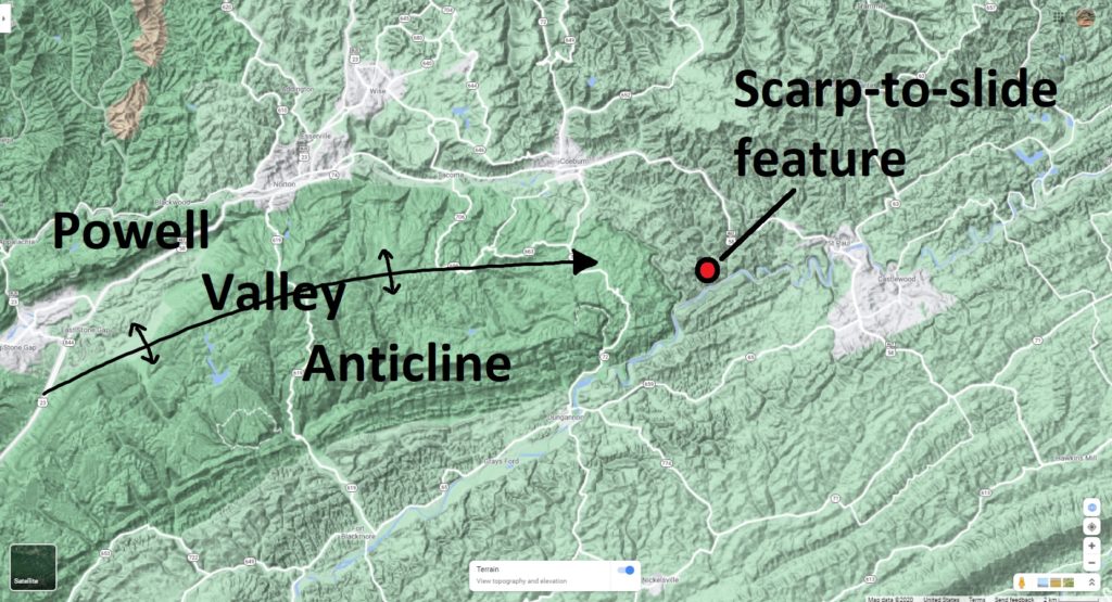
These Wise County coal spoil slides are located on the northeastern plunge-out of the Powell Valley Anticline, a prominent ramp anticline structure near the leading edge of the Appalachian sedimentary fold-thrust belt. Coal measures in this part of Wise County occur in Pennsylvanian-aged strata, which have been extensively mined throughout the area. The scarp-to-slide feature is located at 36.891774N 82.390019W.
You May Also Like
“Blowout” landslides and the lidar signature of extreme Appalachian rainfall events
A mid-1800s description of landslide topography meets 21st century lidar at Split Mountain, Haywood County, North Carolina
Pleistocene Coastal Plain sand dunes and the value of pattern recognition in LiDAR interpretation
-
Interesting “sideways” movement of a large sandstone blockslide
Philip S. Prince
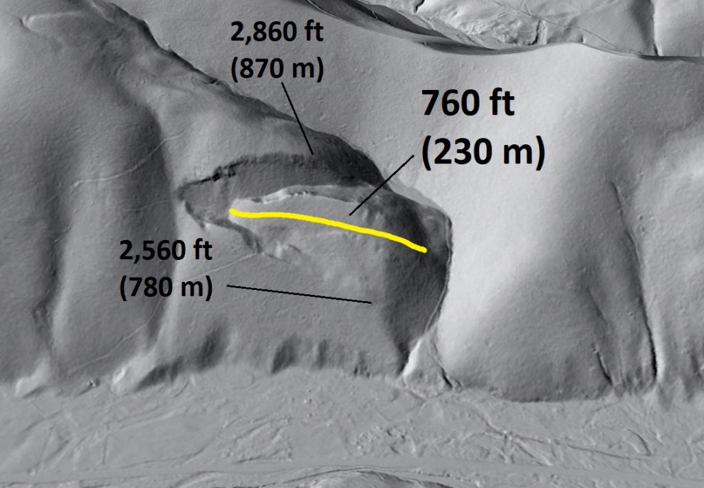
A large sandstone blockslide in Highland County, Virginia presents an unusual appearance in LiDAR hillshade imagery–it appears to have moved sideways across a slope instead of directly down the slope. The slide is entirely concealed by forest cover. It is located at 38.297776N 79.763373W.
The slide has occurred in the thick sandstone sequences of the Foreknobs Formation, whose shale interbeds may have contributed to this failure. The white mobile homes visible at the base of the slope in the GIF above give a sense of the scale of the slide, which is about 760 feet (230 m) long. The upslope scarp is about 300 feet (90 m) above the lower right toe of the slide.
A rotated Google Earth view shows that movement of the slide was indeed oblique to the most direct downslope path, with the slide mass traveling down an inclined plane into the steep stream valley towards the observer.
The slide could be regarded as a wedge failure, with the intersecting failure planes appropriately oriented to allow the slide block to travel towards the open stream valley.
The narrower downslope failure plane likely dips back into the slope to prevent the slide mass from spilling out and taking the steeper path towards the large valley at left in the image. Movement is thus obliquely downslope, with the slide mass “cradled” by the intersecting surfaces to keep it on its atypical path.
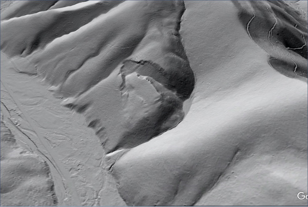
Movement of the slide has destabilized upslope areas of the mountainside, where cracking is visible in the hillshade imagery. The first set of cracks upslope of the slide show the same orientation as the slide’s scarps. They are highlighted in yellow in the GIF below; its resolution should support zooming in.
The uppermost set of cracks near the mountaintop, shown below, appears to be open fractures that may collect surface drainage. The cracks are 2,100 ft (640 m) ground distance from the upslope scarp of the slide, and 500 ft (150 m) above it. The crack system is 370 feet (113 m) long.
While the “sideways slide” is definitely one-of-a-kind in this region, another slide to the north appears to show the early stages of similar but less dramatic oblique movement. It is circled in yellow below, and is just under 1 mile (1.6 km) from the sideways slide.
This slide occurs in the same bedrock units and may share enough structural characteristics to fail under similar circumstances. Both the left and upslope scarps show extension, with compression occurring along the right edge of the slide to produce an overall clockwise rotation.
The sideways slide and its neighbors show the significance of weak and specifically-oriented releasing surfaces in controlling slope failures in the Valley and Ridge, particularly where large, strong sandstone sections are involved. The Foreknobs Formation hosts numerous huge blockslides, some of which were highlighted in this post and this post. As with the sideways slide, these features are nearly invisible without LiDAR-derived imagery and have previously escaped detection!
You May Also Like
Lidar imagery reveals details of debris flow movement in the eastern Blue Ridge Mountains of North Carolina
Erosion and scour in sandbox model debris flows (microbeads and cohesive substrate)
A mid-1800s description of landslide topography meets 21st century lidar at Split Mountain, Haywood County, North Carolina
-
LiDAR reveals the cloth-like appearance of a “wrinkled” translational landslide
Philip S. Prince
The Virginia Valley and Ridge hosts plenty of amazing landslide features, but this wrinkled translational slide in Botetourt County, Virginia is particuarly eye-catching. It reminds me of the wrinkling that might occur in a thin layer of cloth pushed along a smooth surface–something like pushing a napkin or tablecloth along a tabletop. The slide is located at 37.746443N 79.859919W at about 2,000 ft (610 m) above sea level.
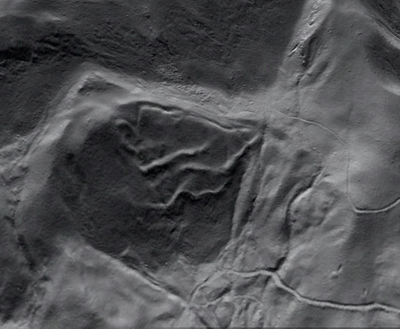
This feature is probably best described as an intact rockslide or blockslide, as it involves a very thin Silurian-aged sandstone layer that has moved downslope. The “wrinkles” are anticlinal folds associated with small thrust faults in the slide mass. The sliding sandstone layer is definitely quite thin compared to the overall dimensions of the slide, creating the narrow folds. Movement on closely-spaced joints in the sandstone layer allows it to fold on the surface without completely shattering, permitting the cloth-like appearance to develop within a layer of rock.
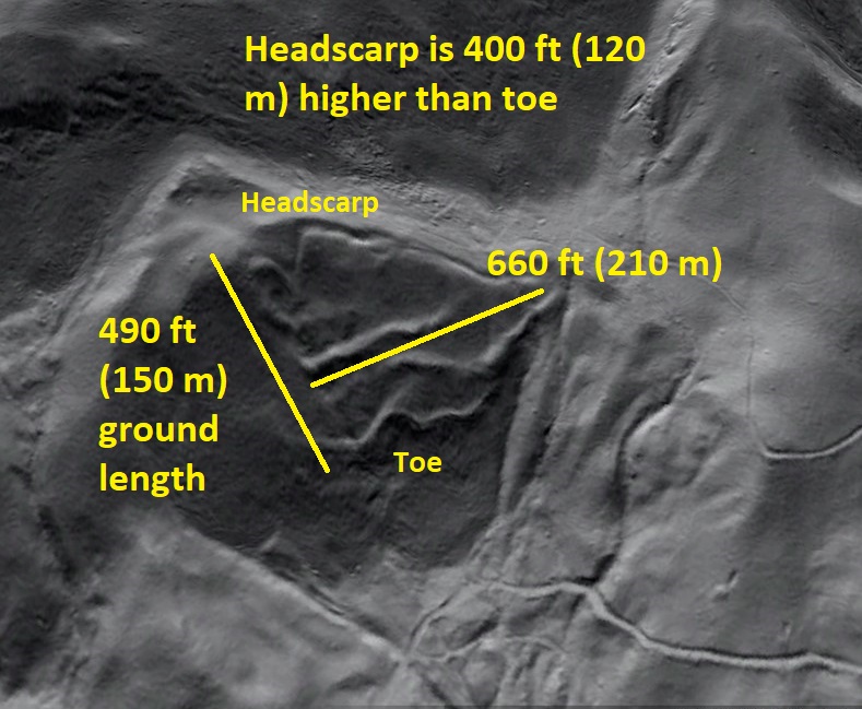
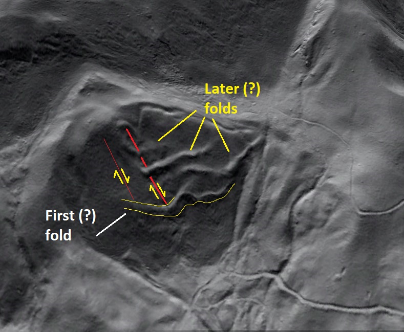
The conceptual diagram below gives a general idea of the type of movement and deformation that creates the wrinkles. They form as the slide “telescopes” onto itself. Dimensions are exaggerated in the drawings, and a notable feature of the real slide is that very little downslope movement appears to have occurred–in other words, there is only a small gap between the headscarp and the slide mass. For this very small amount of movement to create a number of obvious folds, the sliding sandstone layer must be very thin.

The diagram proposes that the lowermost fold develops first. I cannot confirm that this was the actual sequence of events, and I think a geologist could argue for it being first or last. Details of the lowermost fold (which I call the “first fold” in upcoming images) suggest an interesting style of movement within the lower parts of the slide. It appears that the slide mass may have wedged under the first fold in backthrust-type motion, locally arching it and creating a bulge that passes underneath the first fold.
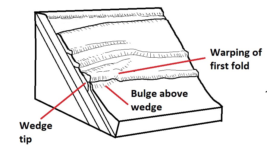
This pattern of movement would explain the very steep upslope side of parts of the lowermost fold, along with the bulge that passes beneath the fold at an angle. In motion, the sequence might look something like this:

I have observed several other thin translational slides in the region that appear to show wedging or backthrusting at their downslope end. Thinness appears to be necessary for the geometry to develop; thicker slides never show it, and a forethrust would likely develop in a thicker slide before noticeable wedge/backthrust motion could occur. As with all of the other Valley and Ridge slides I have written about, age, duration, and sequence of the slide’s movements are completely unknown.
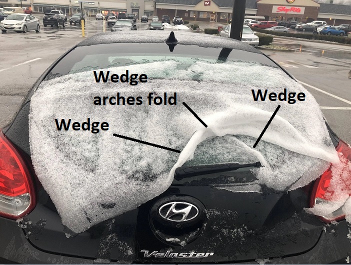
To reach beyond the cloth analogy, a similar type of movement can be observed when a thin layer of snow slides down a car windshield and piles up against the windshield wipers or hood. I actually Googled “snow sliding down car windshield” and was rewarded with a decent match, found at this link. Interestingly, wedge/backthrust features are present, and they appear to arch earlier folds. Movement here is somewhat different, however, due to the “scissor” motion of the snow sheet, which created two overlapping frontal folds (see the GIF below). The original poster of this image also used the cloth comparison for the snow sheet.


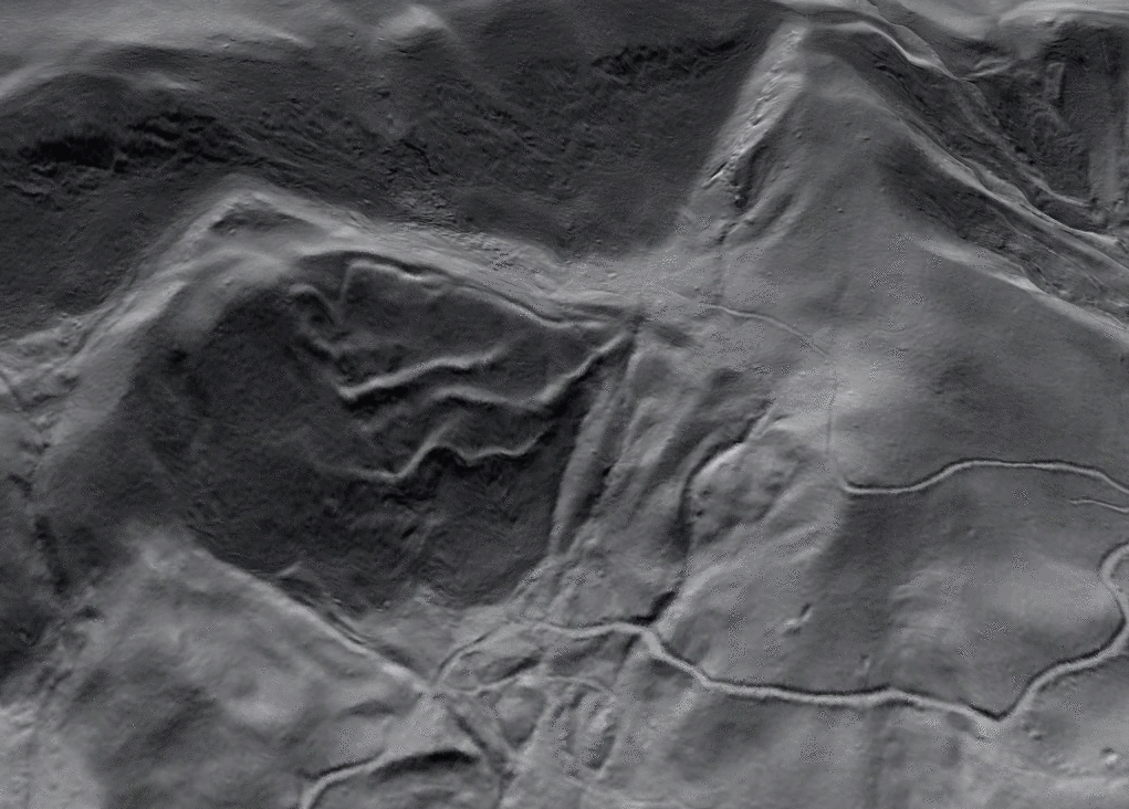
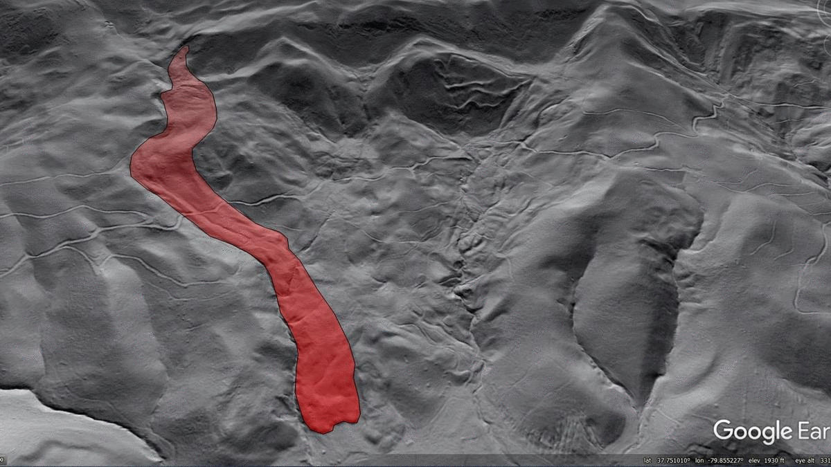
The wrinkled rock slide shares the mountainside with an equally impressive rock avalanche feature just 2,000 ft (650 m) away to the southwest. The rock avalanche moved downhill in a very different way, but it resulted from failure of generally the same part of the layer sequence, although it likely involved more sandstone layers than the thin one that produced the wrinkled slide. The wrinkled slide is visible above and just right of the center of the image.
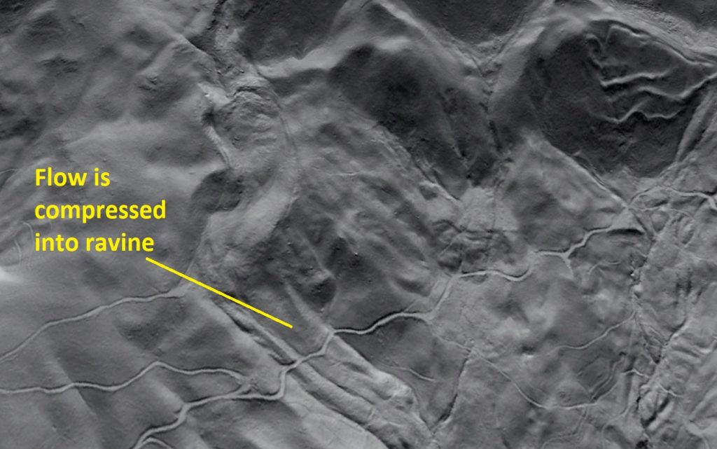
The rock avalanche feature looks like cake batter moving down the slope. It traveled 4,100 feet (1.3 km) overland from its source to the floodplain at the base of the slope, descending about 1,200 feet (365 m). Interesting flow features are visible within the deposit, particularly along the edges of the feature and where it was compressed into a narrow ravine. They are probably described by specific terminology that I admit is unfamiliar to me. Some spillover of material from the flow may also have occurred, but this may also represent earlier flow events.
The entire area between and downslope of the wrinkled slide and the rock avalanche is mantled with older landslide deposits. An older and more degraded rock avalanche feature also appears to pass by the right edge (northeast edge) of the wrinkled slide.
All of these features are testament to the very dynamic slope history of this part of the Virginia Valley and Ridge. Instability is inherent to these slopes, and is probably a combined result of the types of layered rock present on the slopes, the orientation of the layers relative to the slope, and the increase in topographic relief in the area due to incision by streams of the James River Basin. Paleoclimate may have contributed significantly to slide development, and seismic events can not be ruled out as a contributing factor. The collapsing Glen Wilton and Callie iron mines are located 2 miles (3.3 km) northeast along the same ridge, and these features demonstrate possible effects of large-scale, poorly planned engineering on these slopes.
As usual in this part of the Appalachians, all of this is completely invisible without LiDAR-derived imagery!
-
Where Did That Boulder Come From? A LiDAR Perspective On A Large Appalachian Rockfall
by Philip S. Prince, Virginia Tech Active Tectonics and Geomorphology Lab
Large boulders are a common feature on hillslopes throughout the rugged portions of southern Appalachia. “Large” is a relative term, but boulders consisting of over 10,000 cubic feet of rock (a boulder 50 ft x 30 ft x 10 ft = 15,000 cubic feet, for example) can be found in association with a wide range of rock types, river systems, and their associated landscapes. I have always wondered about the possibility of finding the specific outcrop source of large boulders, which is very difficult in the field due to vegetation and continued evolution of the cliff line after a boulder falls off and makes its way downhill. Using LiDAR-derived hillshade imagery of a portion of the Blue Ridge Escarpment in western North Carolina, I recently came across a particularly large boulder that appears to be traceable to a scar on cliffs hundreds of feet further up the slope.
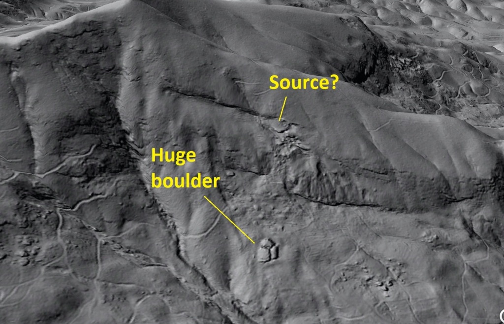
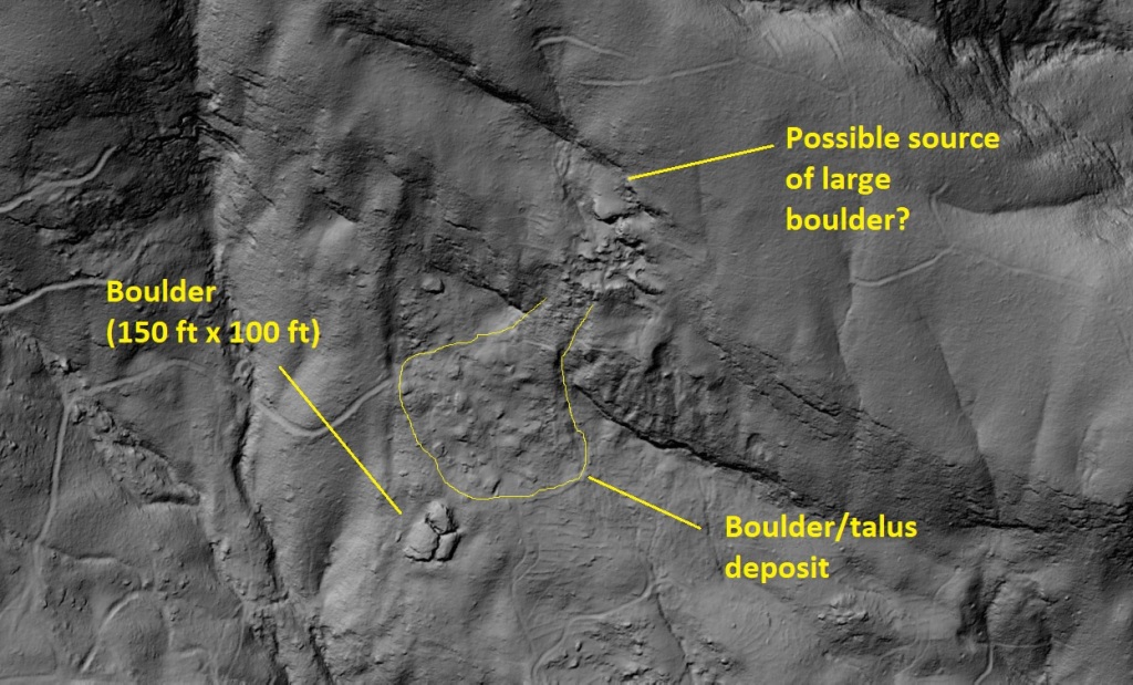
Images like the Italy and Colorado examples near the end of the post keep me interested in looking for surface evidence of a boulder’s trip downhill. I have yet to find success in southern Appalachia, but this potential boulder-and-source relationship is still pretty cool! Even though the boulder looks small, it is 150 ft x 100 ft across its exposed surface, and is probably 20 ft thick or more. See end of post for data source. 
This GIF is featured again below, but it may be useful to pick out features in the perspective image above. This is one big boulder. It is ~150 ft long and ~100 ft wide, and has cracked into three pieces. I don’t know how thick it is, but its survival during its trip downhill and trends in area geology would suggest it may be 20 ft thick or more. Assuming it is 20 ft thick and comparable to granite in composition (it is gneiss), it would weigh 50 million pounds (23 million kilograms). This estimate is derived from calculating the rock volume (150 ft x 100 ft x 20 ft) and multiplying by the weight of 1 cubic foot of granite (168 pounds).
This boulder is seriously large. I can’t estimate thickness, but it is likely considerable given the survival of the boulder and the nature of bedrock in this area. The small boulders in the talus/fan deposit are still impressively large themselves. The shape of the boulder is notable, as its sides meet at angles consistent with fracture and joint intersections visible in the landscape as marked below.
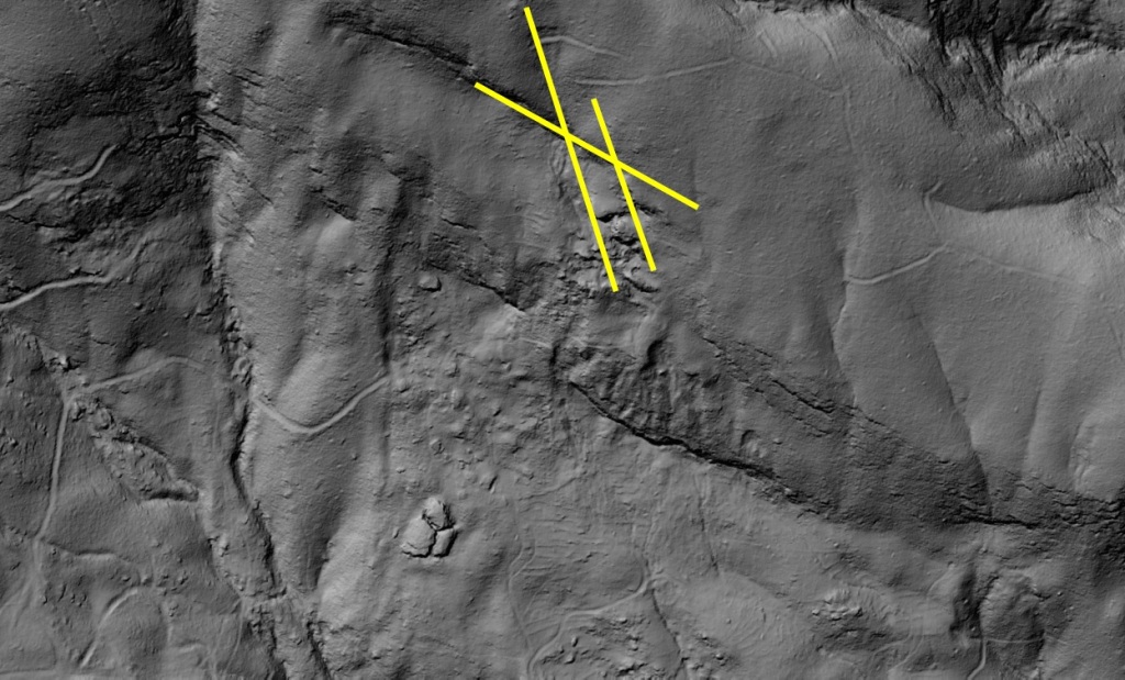
Rockfalls and landslides frequently release along the intersecting joint surfaces and foliation (layering) surfaces in this region. The yellow lines highlight release surfaces, and these zones of weakness can be seen elsewhere in the landscape. Note how the angular outline of the boulder (just down and left of center) resembles the angles between the yellow lines. I thought this particular mega-boulder might be big enough to have left an identifiable scar where it separated from the mountainside. Looking upslope, there is indeed a potential source area that is the correct size and shape to be the boulder’s previous location. An outline drawn around the boulder fits the potential source quite well, although the cracking of the boulder has increased the size of its outline slightly. Bedrock layers visible in the image tilt downslope, setting the stage for such a large chunk of rock to slide off.
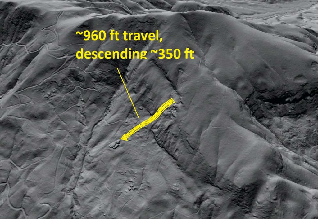
An outline drawn around the boulder matches the potential source nicely. The cracking has made the present outline a bit larger, and a minor size reduction would fit the potential scar even better. I have not visited this location in the field, so I can’t confirm that the scar is indeed the source. I think this would still be very difficult because the potential source area is not a distinctly different layer of rock from areas below it. The intersecting fractures that shape the boulder are also present throughout the landscape, so in theory many areas along the cliff line could be the source. Even so, the matching size and shape of the boulder and potential scar, along with the appearance of the slope beneath the scar, make good evidence for a positive identification of the boulder’s source.
Assuming the scar is indeed the boulder source, the boulder traveled ~960 ft (just under 300 m) over the ground surface, descending ~350 ft ( about 110 m). The boulder appears to have rotated clockwise slightly during its travel. I am always amazed that boulders like this do not completely break apart during their slide. This one did not experience freefall off of a cliff, but its path was far from a perfectly smooth plane.
Travel is significant, but is only a portion of the topographic relief in this steep landscape. Small divots in the land surface at the far right of the image are small landslide scars. It would be interesting to dig a trench on the downhill side of the boulder to see if it disrupted the soil ahead of it during its trip down the slope. Charcoal caught up in the disrupted soil might be useful in setting limits on the age of the boulder movement, depending on how young or old it actually is. Because the feature is located on private property, this probably won’t ever happen!
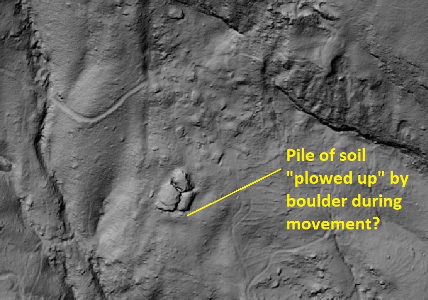
Images like the one below would suggest that the movement of a boulder of this size over a soil- or rock debris-covered landscape would leave a track. I gather the boulder shown below bounced and rolled; the big example above almost certainly slid. I can certainly visualize the indicated feature being a pile of soil and rock fragments “snowplowed” by the boulder, but field inspection would be necessary. The potential pile is still really big, and might be too large for hand excavation to show much. 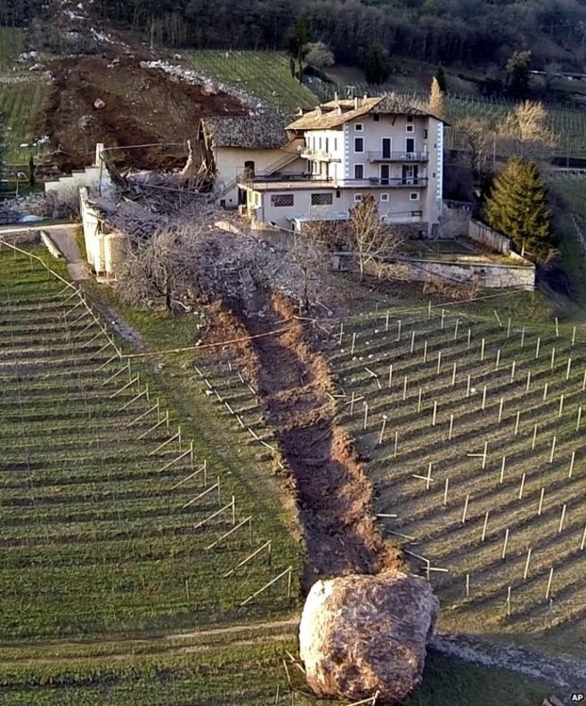
Image source here. The link shows several other images of this event, as well as a shot of an older boulder that followed the same path. The big boulder discussed in this post would probably be the size of the building, if not larger. I have always been interested in the track the boulder shown here has left in the soil. Such a feature would not last long in the rainy southern Appalachians, but could you find any evidence of the soil disruption with excavation? 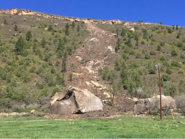
Another good one from Colorado, sourced here. This boulder took an interesting track downhill and certainly deformed the soil where it came to rest. People can be seen at left for scale. This is one is still much smaller than the North Carolina boulder in this post. The boulder is composed of gneiss, one of the tougher high-grade metamorphic rocks in this region. Pennsylvanian-aged sandstones further west in the Appalachian Plateau can produce even more impressive boulders, and all thick-bedded, quartz rich sandstones in the sedimentary Appalachians have the potential to fall apart in enormous chunks that survive downslope transport. As far as I know, there aren’t any recorded instances of these massive boulders moving, and most are just a normal part of the landscape and forest. In most cases, I don’t think its even clear if each boulder moved rapidly in one event or gradually crept down the slope.
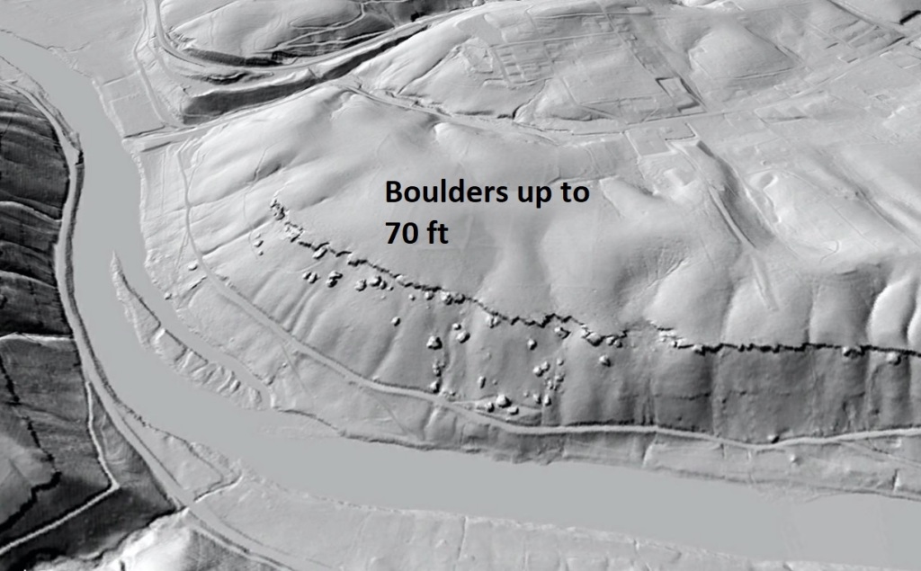
Mississippian-aged sandstone cliff “dripping” boulders (which are still huge) above the Greenbrier River near Talcott, West Virginia. 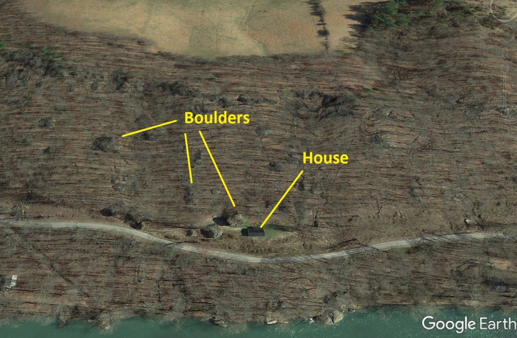
The boulders are just a regular part of the landscape. This house is located on the flat “pad” just below center of the LiDAR image above. In this case, it appears that the house was mistaken for a boulder during LiDAR processing, which usually removes buildings (you can see building pad outlines near the top of the image). Google Earth shows that there are two boulders next to the house. The LiDAR image shows three. In the case of the North Carolina example, I certainly imagine a rapid, single event that would have been very impressive to watch.
LiDAR data source: QL1 lidar data acquired by NC Dept. of Public Safety, raw point clouds assembled and processed by Corey Scheip of the NC Geological Survey Landslide Hazards Program.