Lidar imagery reveals details of debris flow movement in the eastern Blue Ridge Mountains of North Carolina

by Philip S. Prince

Lidar-derived imagery is a remarkable tool for showing how rock, soil, and woody debris moved over the landscape during old debris flow events. Understanding how this material moves is a key aspect of understanding present-day debris flow hazard. Lidar imagery provides a way to track downslope material movement of old flows that is otherwise difficult or impossible to see in the field, which is particularly significant in forested Appalachia. This post highlights some interesting debris flow styles and paths now hidden by vegetation in Pisgah National Forest in Transylvania County, North Carolina. I have tried to label relevant features without obscuring details of the deposits, which are quite subtle but notably distinct from the rest of the landscape once you see them. The GIF below uses a transparent polygon to highlight a flow path and deposit on the north side of the Davidson River southwest of Brevard, North Carolina. This one is a good starter, as details of the initial failure and subsequent flow path are reasonably easy to pick out.

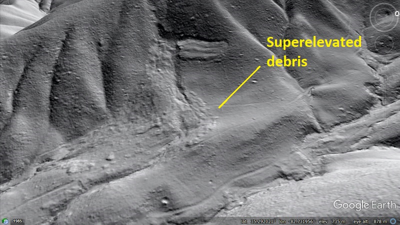
This flow appears to have resulted from the partial breakup of an intact landslide block, much of which did not flow and remains clearly visible as a detached rectangular feature on the slope. For a sense of scale, the intact rectangular block is about 200 ft (60 m) across. Due to the shape of the landscape, the debris flow resulting from breakup of part of the slide block quickly reached the smooth but sloping valley floor, where it spread out before re-channelizing toward the bottom of the image. The flow had sufficient momentum to superelevate (move at an angle to the slope instead of straight down the slope) and bend away from the faint upper channel before the material turned back towards the channel. A faint dashed yellow line highlights the curve in the levee-like deposit edge as it bends back onto a direct-downslope path.

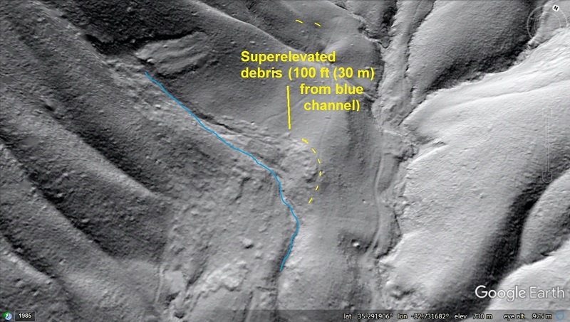
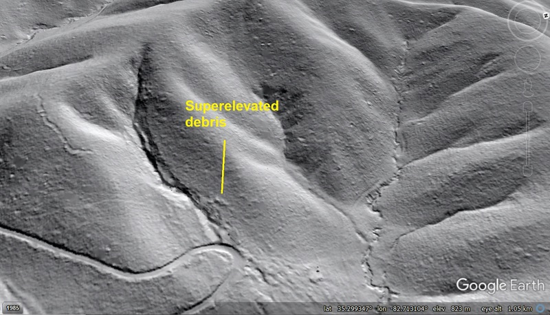
Superelevated debris extends about 100 ft (30m) across the ground surface from the faint upper channel, which is highlighted by the blue line.

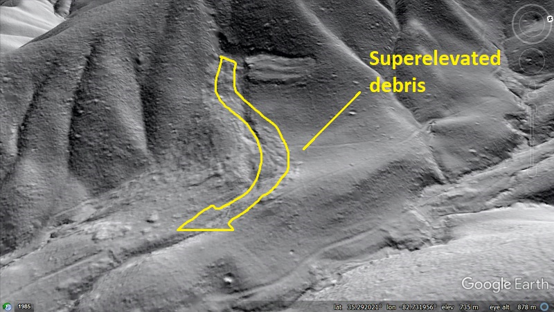
A head-on view (below) gives more context to the superelevated debris, which moved oblique to the slope of the valley before losing momentum and following the slope. The second image offers a basic illustration of how the debris “banked” its way downslope.

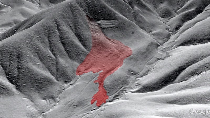
Lobes and sheets of deposited material, along with one large boulder, are visible further downslope. This slide-to-flow was obviously quite fluid and mobile despite the modest relief between the failure point and the sloping valley bottom. After traveling overland in the area shown above, portions of the flow re-channelized and continued downslope. The deposit terminates at a ground length distance of 1.180 ft (360 m) from the failure point, having descended about 265 ft (80 m). The transparent polygon in the image below covers the full extent of the deposited material visible in lidar.

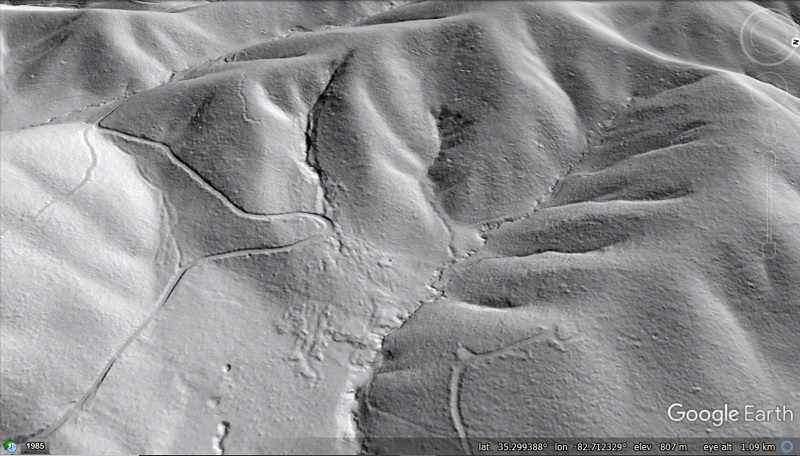
2.2 miles (1.3 km) to the east, another subtle debris flow deposit is visible spreading across a gently sloping valley floor. The GIF below shows the extent of the deposit, which resulted from a flow originating in a small channel upslope. No clear initiation zone is visible above the head of the channel, suggesting the flow began within colluvium stored in the small channel itself. The deposit highlighted by the transparent polygon is about 280 ft (85 m) wide at its widest.

This flow also occurred in reasonably modest topography, descending about 230 ft (70 m) over a ground length of 1,000 ft (~300 m) from the apparent initiation zone to the toe of the deposit. Near the upper end of the polygon, a line of superelevated debris is visible on the otherwise smooth hillslope. This material was likely deflected onto the slope by the slight bend in the to the left of the superelevated debris as shown in the image below.

While the deposit from this flow is more subtle than the previous slide-to-flow feature, it is definitely visible once you know it’s there. The lowermost portions of the deposit stand out nicely against the comparatively smooth valley floor. Much of this deposit is draped across a faintly convex area, which is visible just below the logging road switchback that cuts into (and obviously postdates) the deposit.

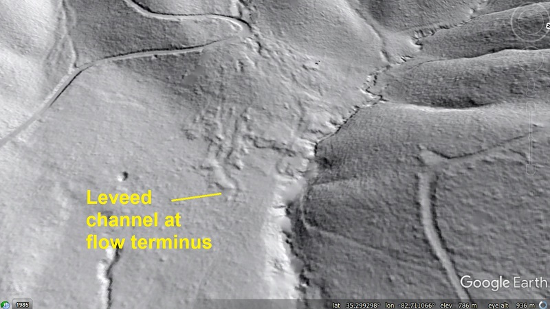
The leveed channel at the tip of the deposit is particularly interesting, with the outlet for fines and flowing water clearly visible.

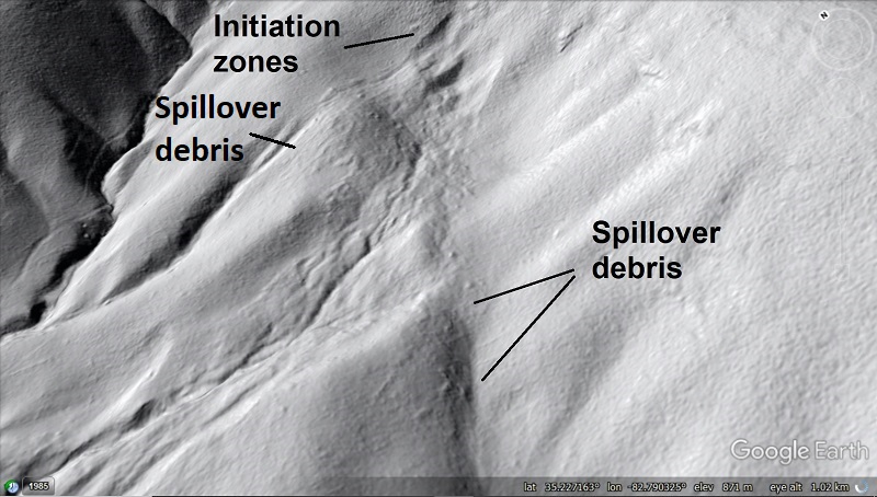
About 6 miles (~10 km) southwest, a comparatively complex debris flow deposit can be seen on a slightly larger and more rugged hillslope. This deposit spilled out of the narrow, shallow “trough” that steered it in two places, though the bulk of the flow reached the stream below after traveling a ground length of ~1,200 ft (~364 m). The flow descended ~380 ft (115 m).

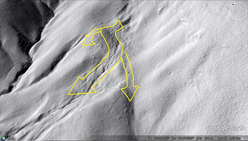
The “spillover” zones result from the unusual topographic shape of the hillslope, where three faint channel heads are located in close proximity to one another. This failure was also quite voluminous; the failure scars are about 25 feet (just over 7 m) deep and 260 ft (80 m) wide. An oblique image (below) puts both “spillovers” into topographic context. The second image uses yellow arrows to give a sense of material movement in this failure. I have actually visited this feature in the field, and the spillover material would not be noticeable without lidar-derived imagery of this (0.5-meter) resolution.

These debris flows are particularly interesting to study because they are distinct from many other debris flows in the region, whose downslope travel is strongly controlled by topographic channels along much of their length. The flows shown here experienced less topographic control and presumably less “bulking up” by collecting soil, rock, and wood along their paths. Despite their lack of extended channelize flow paths, the spread of these flows, along with their mobility in close proximity to their initiation zones, provides an interesting glimpse into the physical dimensions of possible impact zones related to this type of slope failure. The age of these failures is unknown, but they likely occurred in 1916 during an extreme tropical precipitation event in the area. They are completely obscured by forest cover today, and the information about slope failure effects that they preserve would be completely lost without this lidar data set!