-
Moving mountainsides: The giant quartzite landslides of the Macks Mountain area of the Virginia Blue Ridge
by Philip S. Prince
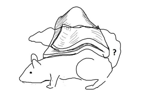
Landslides can be triggered by a variety of conditions or events. Erosional removal of the base, or toe, of a steep slope is a common cause of landsliding, sometimes creating “stop and go” landslides that move episodically when erosion carries away just enough material to create instability. After a bit of slide movement restores the shape of the slope toe, movement stops until enough material is eroded again. The model below shows what this process looks like. Scraping a tiny bit of material from the base of the slope causes an equally tiny movement of the slope. Continual scraping away of material causes the effects of small movements to add up, gradually producing a large and impressively cracked and fractured landslide mass.
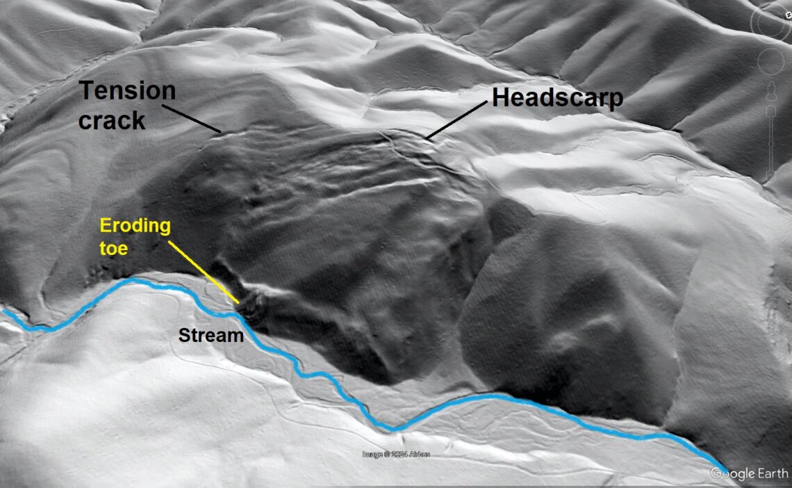
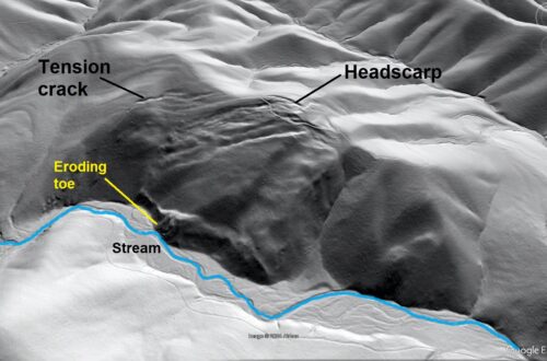
Some interesting real-world slides that appear to result from this type of ongoing erosional toe removal are found in the Macks Mountain area in the Blue Ridge of southwest Virginia (map at the end of this post). The lidar image below shows one such slide, whose appearance can be matched to the later stages of movement of the model shown above. Cracks and fissures extending from the top of the ridge are clearly visible, as is the steep, eroded toe along the stream. The slide is 2,000 ft (600 m) wide. The top of the ridge and head of the slide are about 600 ft (180 m) above the stream below.
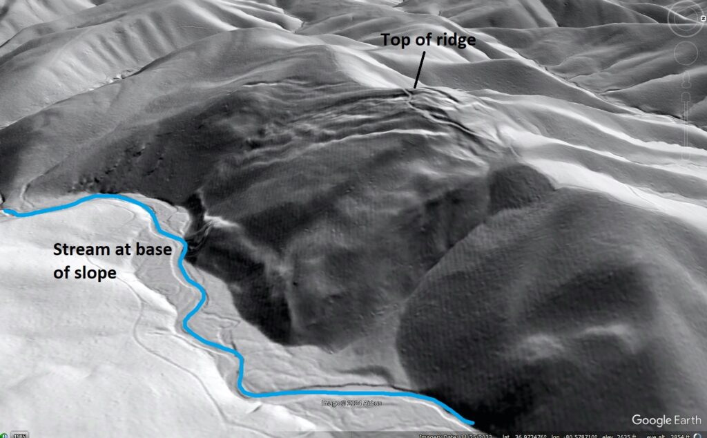
The cracks and fissures at the head of the slide along the ridge crest stand out against the normally eroding parts of the surrounding landscape. The unusually steep eroded toe of the slide, which is in deep shadow in this hillshade image, also contrasts with the even the steepest streambanks in areas unaffected by sliding. At the left side of the image, faint bedrock ribs can be seen on the land surface. These bedrock ribs indicate that layering tilts down towards the stream, favoring sliding.

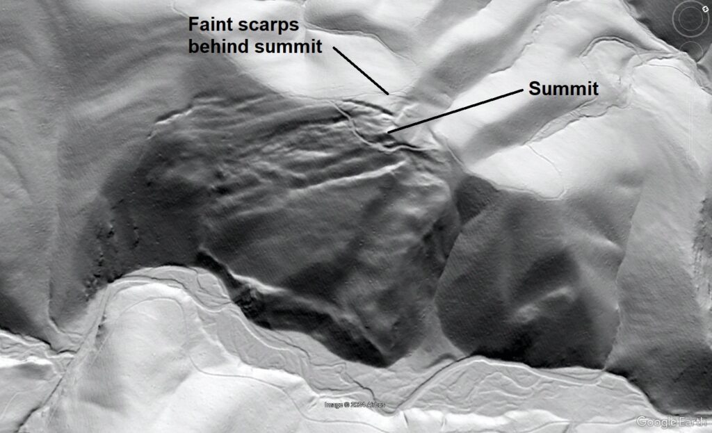
A particularly interesting detail of this slide is the presence of faint scarps or tension cracks behind the summit of the ridge with respect to the stream at the toe. In other words, the actual summit of the ridge is within the slide mass and has lowered and moved downslope just a bit. This arrangement of slide features with respect to the shape of the slope indicates that the slide is thick and is moving on a weak layer or layers deep beneath the surface of the slope.
The geology of the Macks Mountain area sets the stage for numerous huge slope movements like the one shown above. Macks Mountain features rugged topography due to the presence of folded and faulted quartzite bedrock, which is quite hard and resistant to erosion, alongside weaker layers of mica-rich slate or phyllite bedrock. Slate or phyllite cannot support the slope steepness that develops due to the “armoring” effect of quartzite layers, leading to big landslides that slowly feed rock into the eroding streams below. Lidar imagery makes the slides easy to see, but their size and subtlety would make them less than obvious to a ground observer. The example shown below features the characteristics seen in the previous slide.
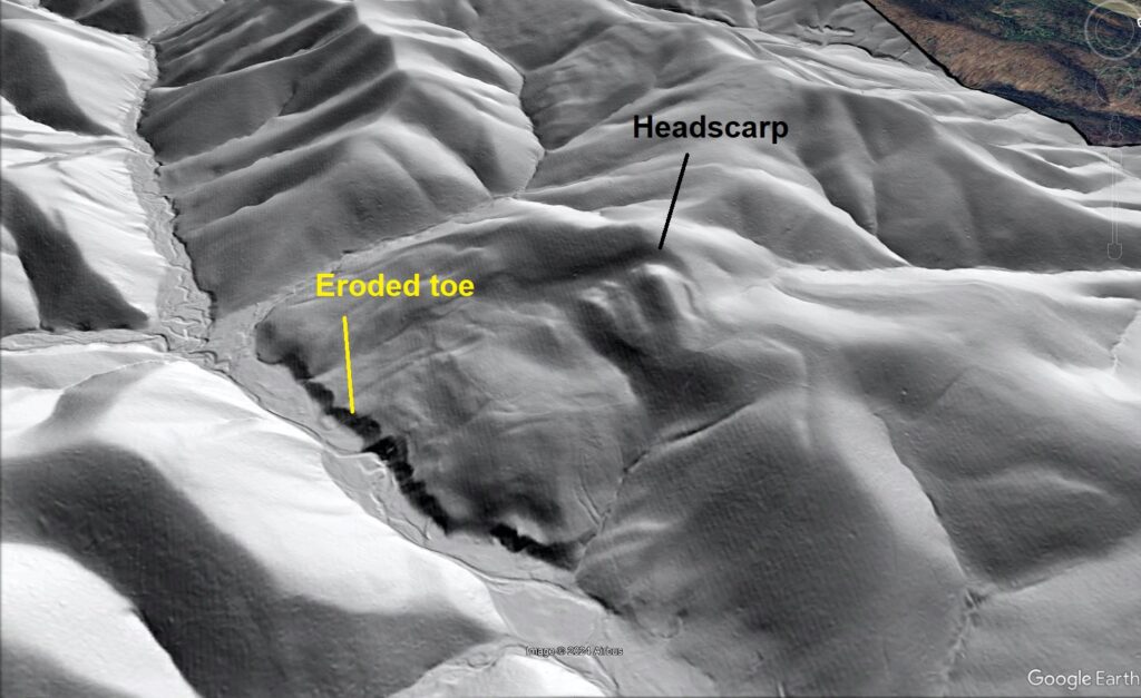
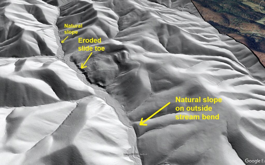
This slide is a bit less crisp and sharp, suggesting it might be a bit older or be in a longer period of suspended movement. Even so, the steep, eroded toe and blocky, lumpy topography below the headscarp contrast nicely with the surrounding erosional topography. The eroded toe area is particularly distinct, and is notably different from even the steepest streambanks in areas not affected by sliding, as seen below. This toe steepness suggests some slide movement is recent enough that the toe has not yet returned to an appearance more like the undisturbed landscape.
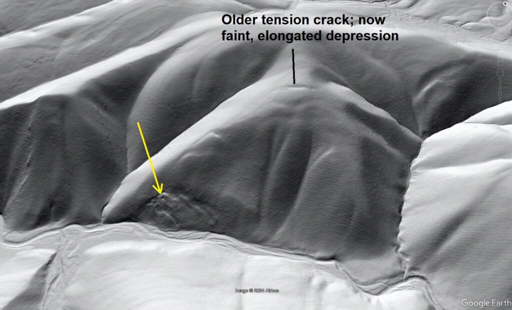
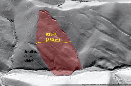
Bedrock-involved landslides like these come in a variety of sizes in the Macks Mountain area. Some smaller slides appear to have destabilized larger areas of the slope, possibly setting the stage for future movement of larger areas. The small slides indicated by yellow arrows below are about 1/4 the size of the first slide in the post, but they have developed for the same geologic reasons.
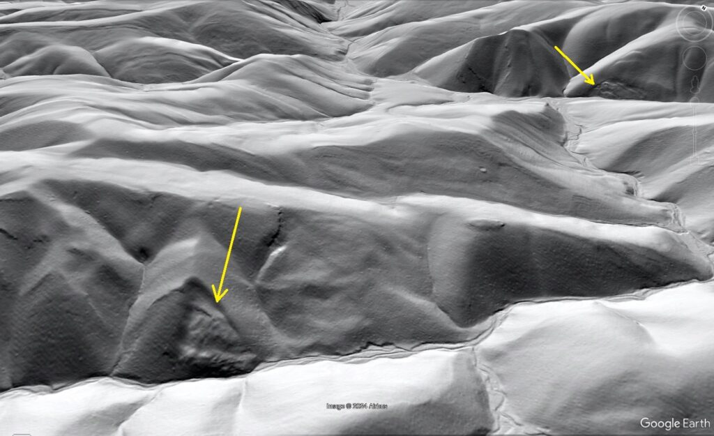
The slide in the background of the image above appears related to older tension cracks well upslope of the crisply defined slides. Now a faint, elongated depression, the upper tension crack suggests that a huge portion of the slope once experienced a tiny amount of movement, and might shift again in the future.
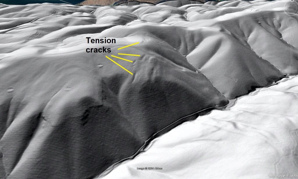
Other old tension crack sets do not have any obvious recent slides associated with them. These cracks also suggest that slopes in the Macks Mountain area exist at the threshold of movement, possibly due to stream incision and relief production associated with the downcutting of the nearby New River. The tension cracks shown below are similar to the example above, though more numerous. A road grade and stream are present at the base of the slope, though no smaller slides are visible. The tension cracks would appear as subtle depressions in the forest today, as soil development has dulled their outlines.
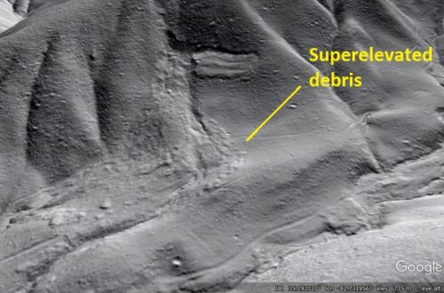
Near this group of old tension cracks, two unusual topographic features are likely the result of the largest and thickest slope movements in the area, although their unusual appearance makes interpretation more difficult. These possible slides are shown below.
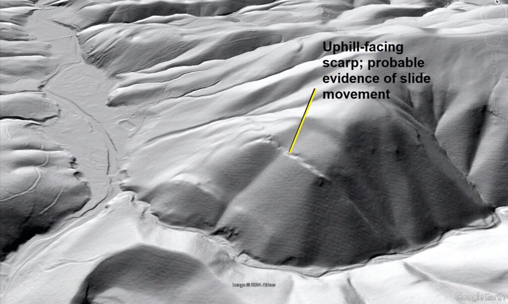
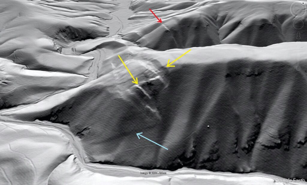
In both images, yellow arrows indicate probable scarps that are significant to a landslide interpretation. In the image above, the light blue arrow shows a likely toe bulge related to faint downslope movement. The red arrow in the background indicates the position of the uphill-facing scarp in the previous image. These features lack the ease of interpretation of the other slides shown, but their features are effectively impossible to explain without slope movement. Uphill-facing scarps and the associated localized surface depressions are very significant. “Typical” sinkholes related to bedrock dissolution do not form in this type of rock, so any surface depression results from a physical gap due to slope movement or excavation by humans. The model below shows uphill-facing scarp development, along with localized sinking of the model surface.
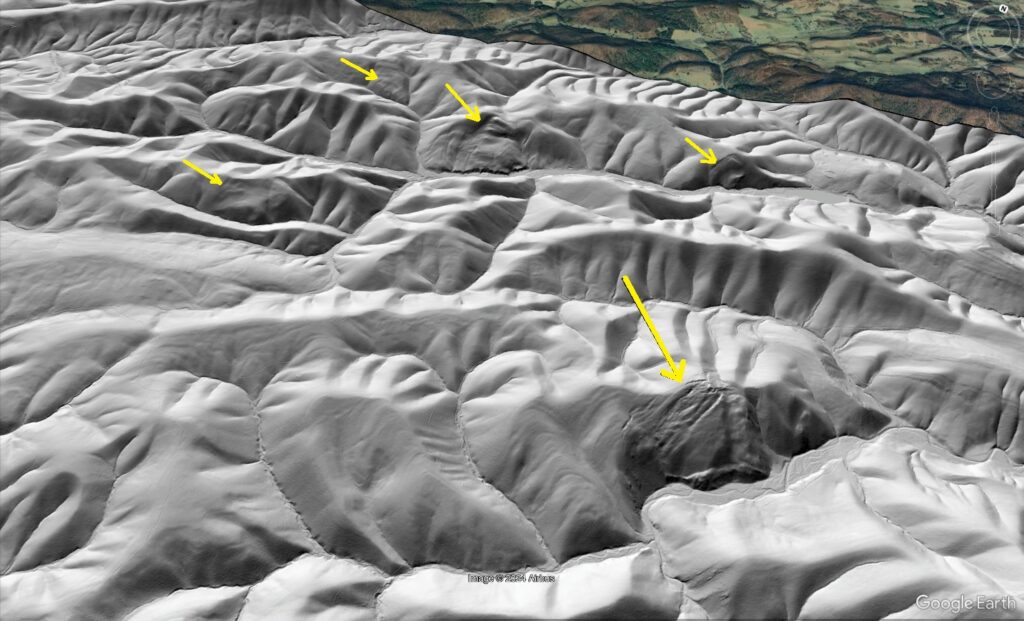
The big “mystery” features do not resemble surface excavation in any way. They are very large, oddly shaped, and have formed in areas with no access roads for the equipment and personnel necessary to remove such large masses of rock. Due to the prevalence of large-scale bedrock landsliding in the area, the “mystery” features can reasonably be interpreted as large slope movements. A zoomed-out view of the surrounding area shows that landslides aren’t hard to find in amongst the ridges of Macks Mountain due to the bedrock character, slope steepness, and likely history of relief production in the area. Yellow arrow point out slides in the image below, which is a nice practice image for pattern recognition in lidar interpretation.
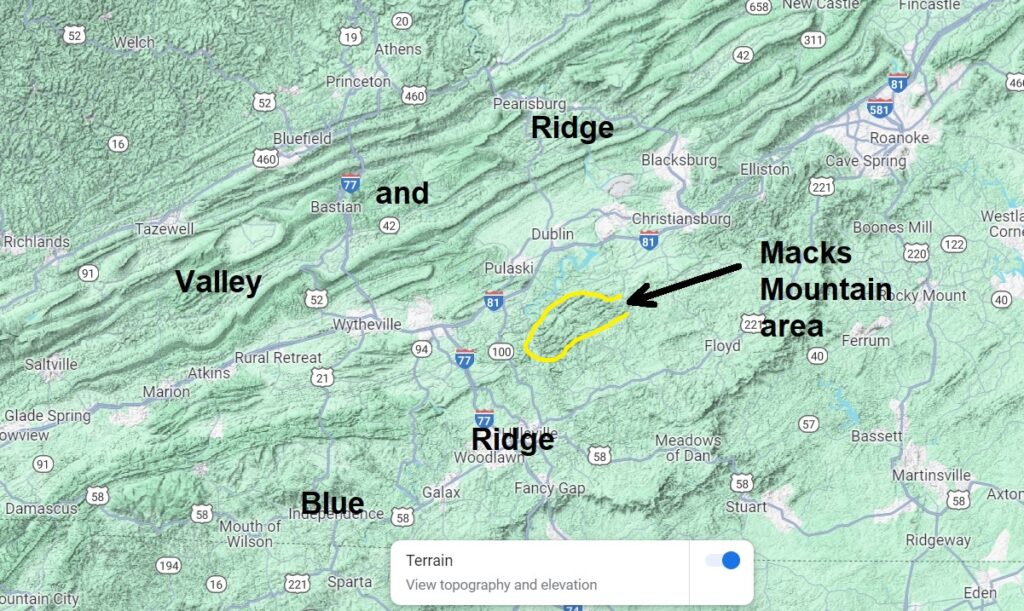
Big bedrock landslides are a common topic on this blog, as they are fundamental feature of many mountain landscapes in southwest Virginia. The most well-known slides occur in the Valley and Ridge, where tilted sandstone layers slide on weak shale layers. Macks Mountain is underlain by metamorphic rocks of the Blue Ridge province, but quartzite and phyllite are just slightly “cooked” sandstone and shale, respectively. Quartzite and phyllite retain the extreme mechanical contrasts of sandstone and shale and behave accordingly in the landscape. The relative locations of the Macks Mountain area and the Valley and Ridge are shown below.
A particularly interesting aspect of Macks Mountain slopes is that none of the slides appear to exhibit large-scale, rapid movement that would be particularly dangerous to people in the area. Topographic evidence suggests the slides just creep along, and may see suspension of movement for very long periods. While they don’t threaten people living nearby, engineering projects would need to avoid the slides. As stream erosion appears to be a driver for their movement, excavation of the toe of slide to build a road or any sort of structure in a stream valley would likely lead to movement. Projects like pipeline construction also need to consider this type of slide, as even slight movement can have catastrophic effects should the movement rupture a pipeline. Fortunately, high-quality lidar imagery makes big landslides like these easy to see in the landscape, supporting good decisions with regard to land use and development.
-
Making lateral spread landslide models with glass microbeads…and lots of shaking!
by Philip S. Prince
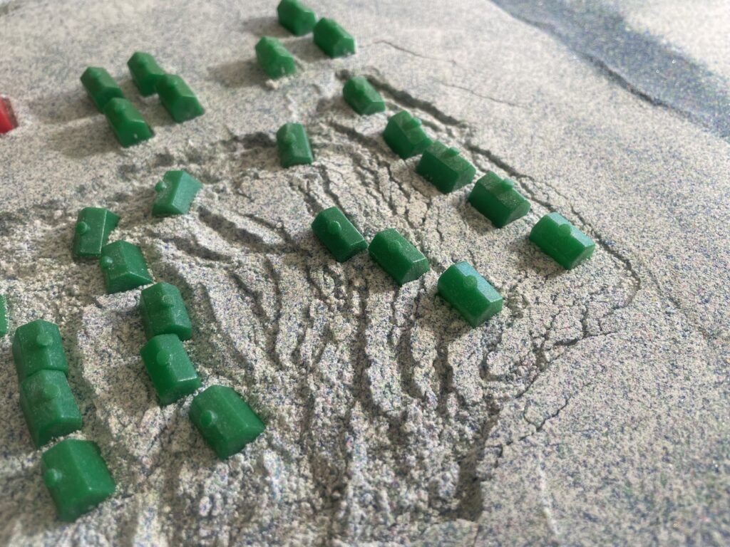
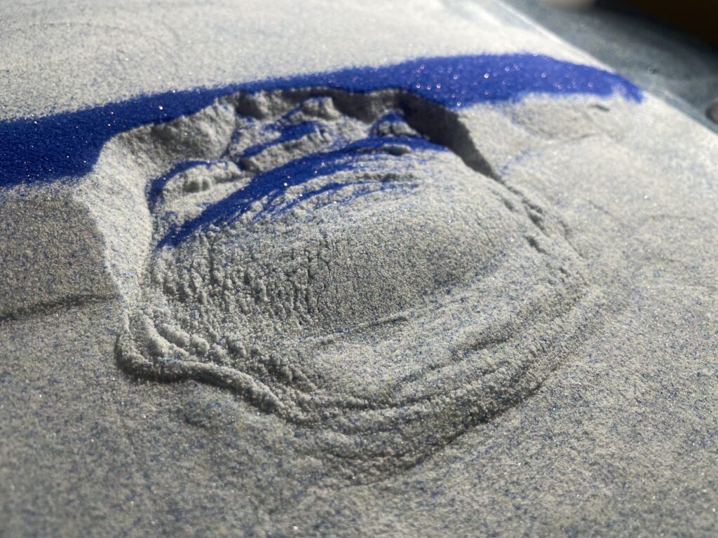
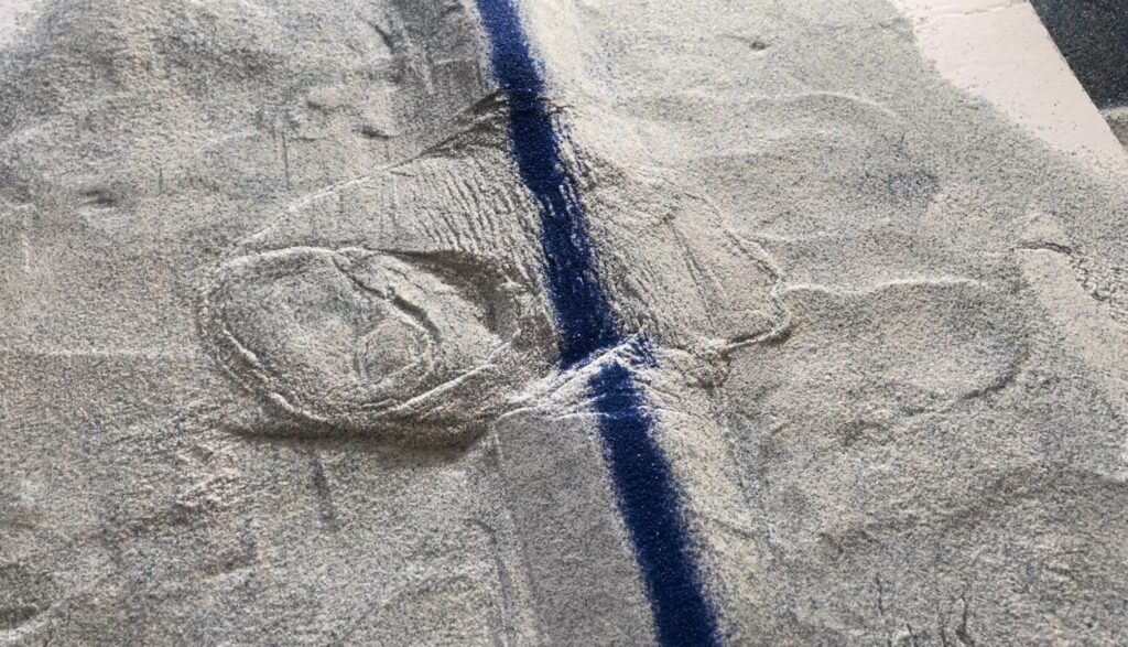
Many aspects of geology are fundamentally related to material movement, but geologists can often only examine the final results of the movement for reasons of physical scale, time, and safety of personnel. Earthquake-related lateral spread landslides are a good example–they create incredibly dramatic landscape damage, but filming one from an appropriate vantage point during intense shaking is nearly impossible. Physically modeling lateral spreads is also problematic because of the soil liquefaction involved; it’s tough to combine dry and wet granular media and keep them (and their properties) separate. An illustrative, and entirely dry, lateral spread model can be made using glass microbeads beneath a cohesive sandpack, which I make by combining sand and flour. During shaking, the microbeads behave like a viscous fluid and deform the overlying sandpack. The images below show one such model I recently made. I decorated the pre-slide landscape with Monopoly houses and hotels, which got caught up in the action.
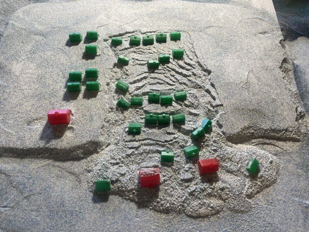
Lateral spread models made in this way are entirely conceptual and illustrative, but they look cool and do reproduce details of ground deformation above a seismically liquefying horizon. A sandpack is constructed over a layer of glass microbeads, and the whole baseplate under the model is shaken to cause the microbeads to “liquefy.” Deformation to the cohesive sandpack above the microbeads is visually interesting, with complex arrays of scarps and rotated blocks, as seen below.
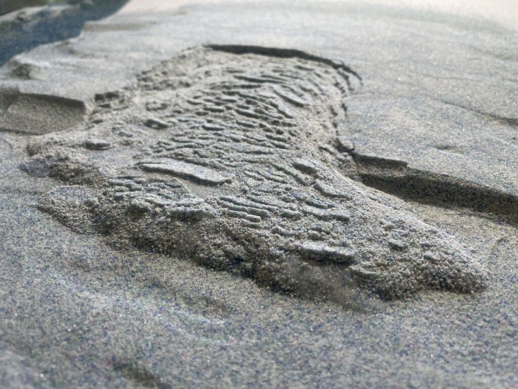
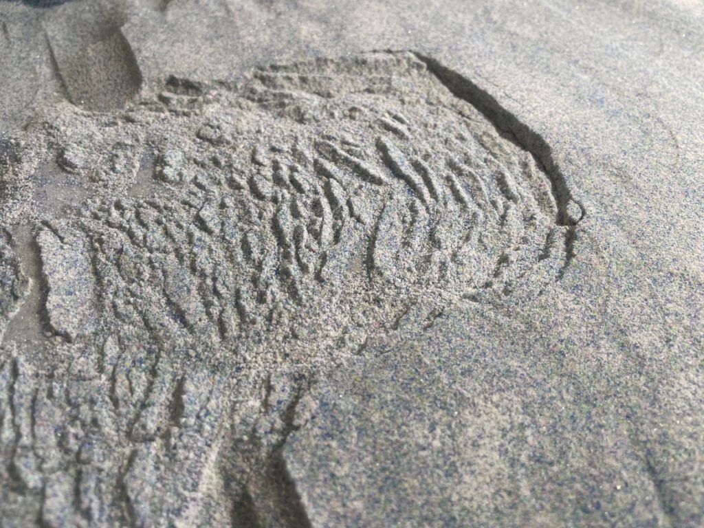
No effort is made to scale the shaking; the model is simply shaken until the microbeads lose strength, presumably due to reduced sliding friction against one another during acceleartion. The in-motion appearance of these model is fun to watch, and is the main thing to take away from this post. The video linked below shows the model above, along with two others. The video shows shaking and failure at 1/2 speed, which is a bit easier to watch.
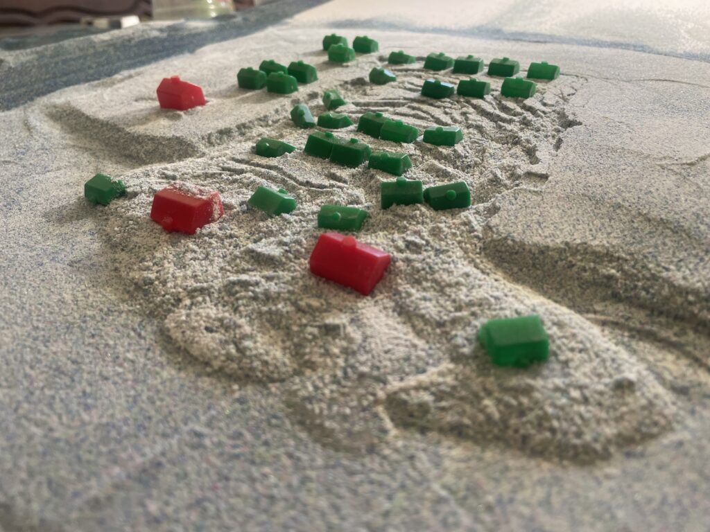
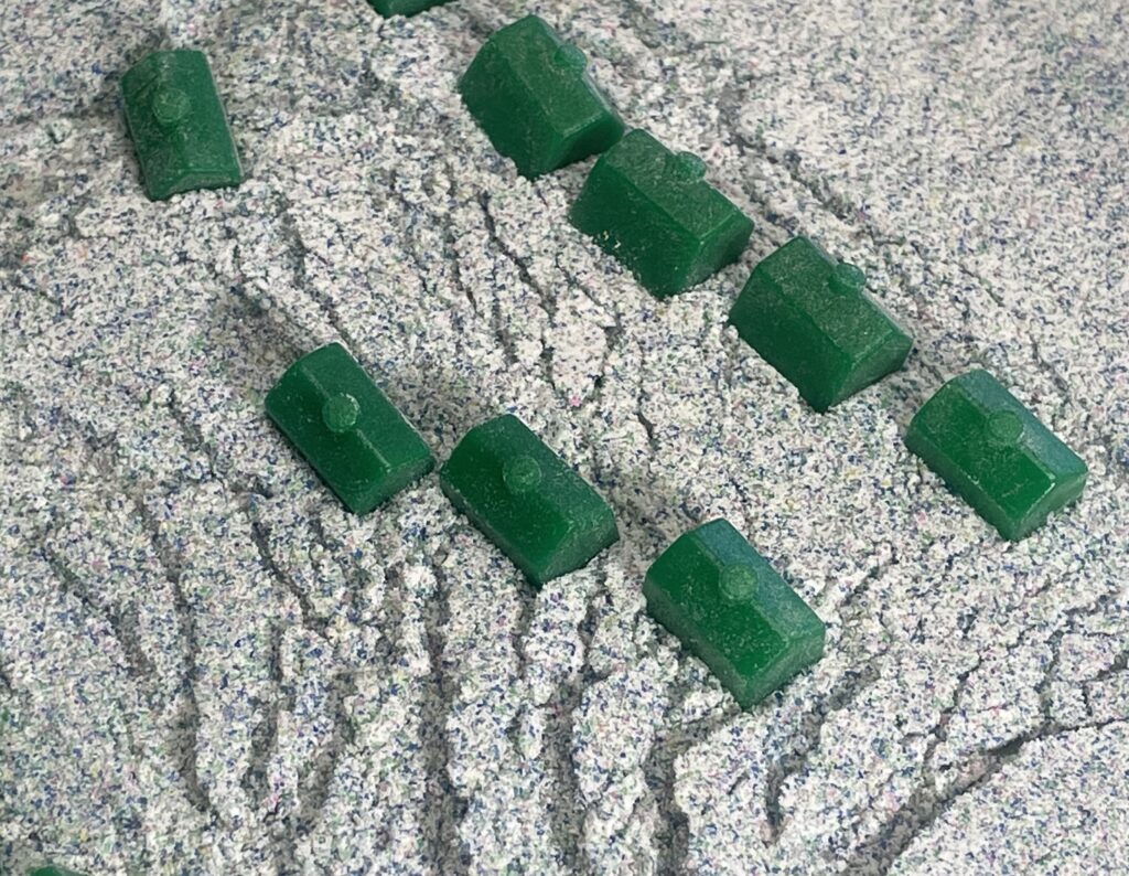
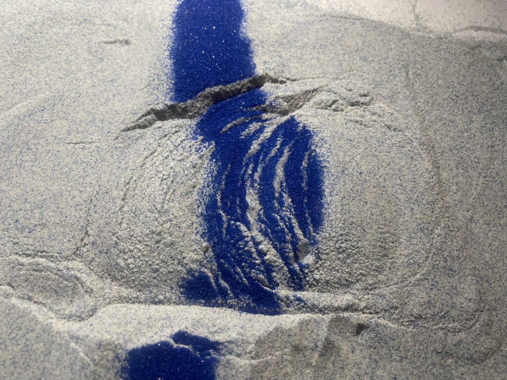
While the frequency and amplitude of shaking are exaggerated to get the desired outcome, the lateral spreads made using microbeads display some realistic details that are useful for students or non-geologists to see and connect to a formative process. Block rotation and tilted or sinking of structures within the spread is one such detail, as seen below.
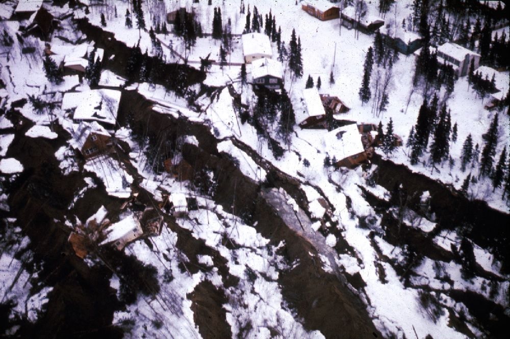
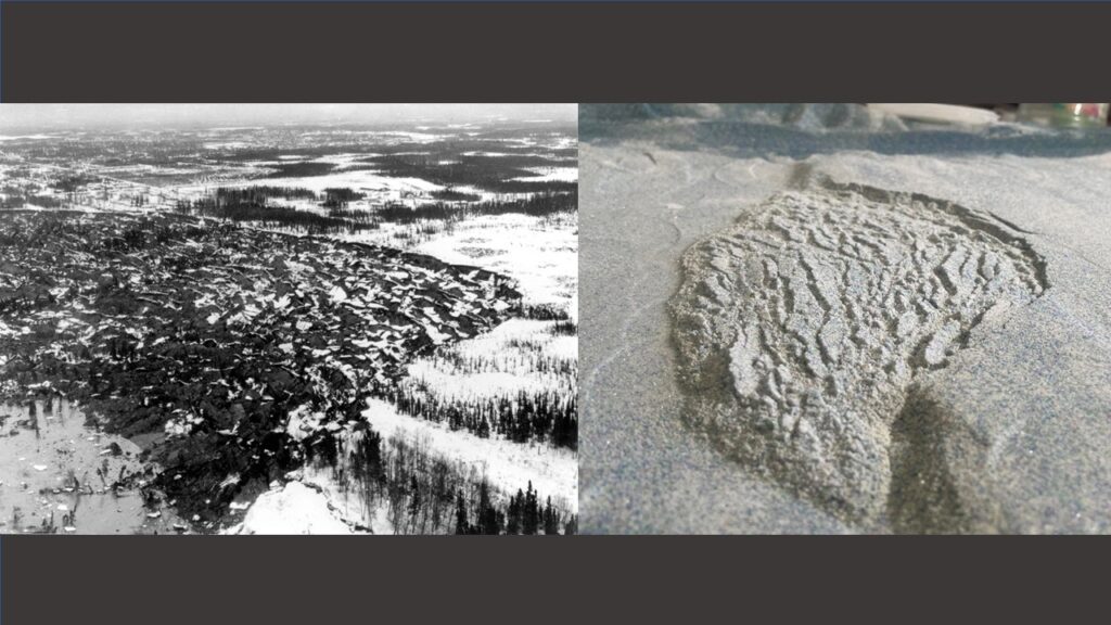
I tried to make these match some of the Turnagain neighborhood images from the 1964 Alaska quake, with acceptable result. The image below is from The Atlantic, I believe.
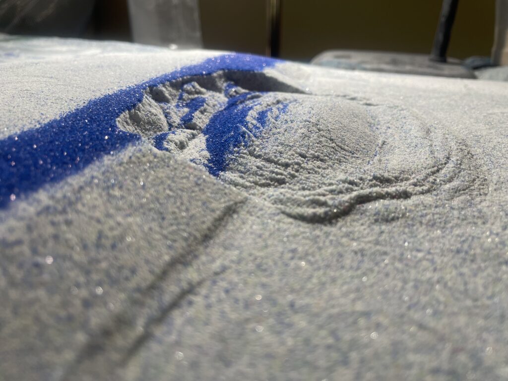
The model lateral spreads also move with gravity and require very, very little slope to do so. Tilting the baseplate only a few degrees will lead to downslope flow. The models shown above used a slightly (3 degrees?) tilted setup and a daylighted microbeads layer (the model starts with a “bluff” below the houses) to create a strongly directional spread. The overall appearance, along with the finer details, can be made to match photographs of real lateral spreads very closely.
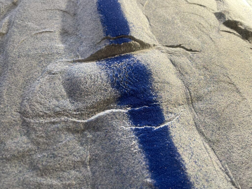
Lateral spreads affecting infrastructure can also be modeled. The experiments shown below induced lateral spreading below a model embankment. Again, with slight tilt or asymmetry, the spread that develops is directional. The arcuate scarps in the model spreads below turned out well.
These models confined the microbeads in all directions, and they “sloshed” significanlty from side to side; this movement is easily visible in the video linked below.
The final geometry of these spreads was remarkably flat, with a gently raised toe bulge and equally low slope slide head. Head and toe reaches this equilibrium geometry when the microbeads layer was at its weakest.
Inducing a lateral spread beneath a symmetrical embankment-type structure with no tilt produced a variety of results, but bi-directional spreading and toe compression are possible. Sloshing was a problem here, too–see the previous video link. Shaking in a single direction meant that the final outcome related to orientation of the embankment to the shaking direction.
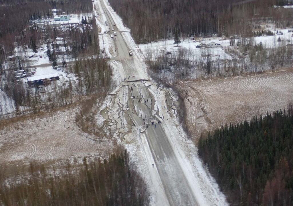
I wanted these models to compare with one of the more widely distributed examples from the 2018 Alaska earthquake, where a road (Vine Road, I believe) experienced a bi-directional spread with two compressional toes. The image below is from the USGS My setup needs more work, but the potential is there…
The obvious drawbacks to these models are the lack of true pore water-induced liquefaction and the exaggerated shaking and sloshing, but these models are easy to set up, easy to break down, and make the connection between shaking, distinct material behaviors, and earthquake/slide-related landforms easy to appreciate. Vibrating the base plate might also produce a good result, but I have not constructed a rig to produce it. If anyone gives it a shot, let me know!
-
Another track left by huge boulders visible with lidar, Big South Fork National River, Kentucky
by Philip S. Prince
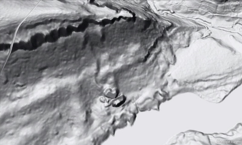
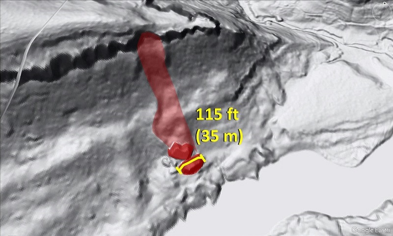
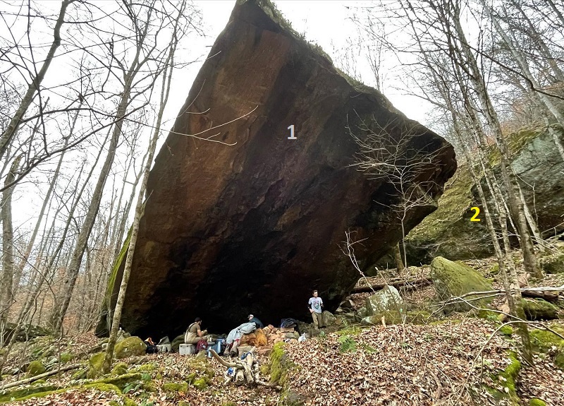
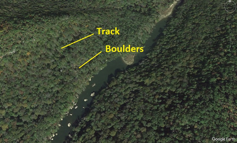
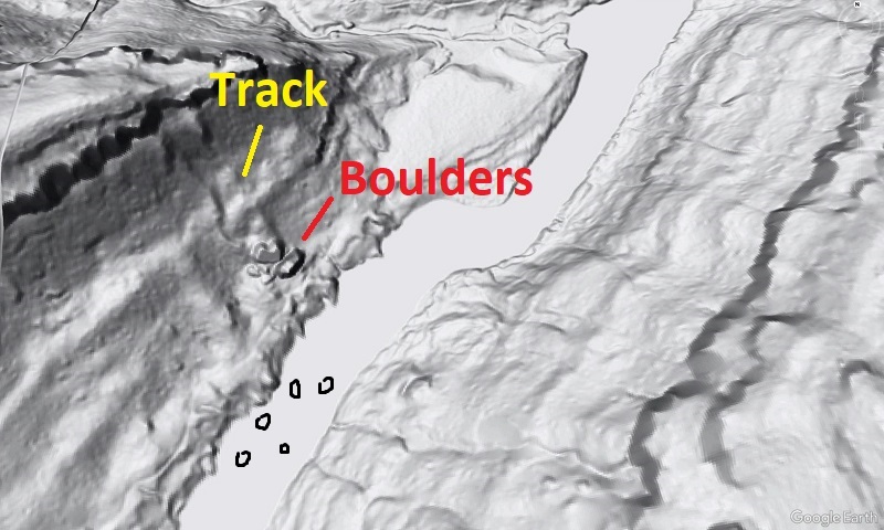
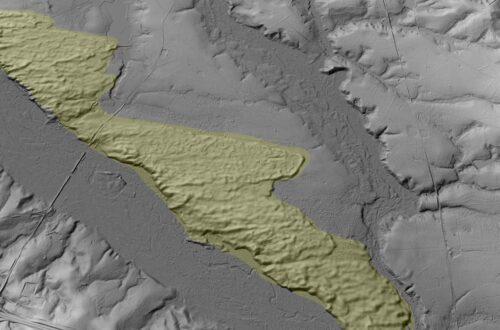
As rugged and/or high topography in Appalachia tends to result from outcrop of particularly hard and weathering-resistant rock, steep slopes in the Appalachians are often home to boulders, some of which are quite large. An interesting aspect of the boulders is that very few have been known to slide or roll into place since folks started recording such things, and they very, very rarely show visible tracks or paths downslope in lidar-derived imagery. The question of how the boulders got to their resting place is legitimate (more on this below), but sometimes, lidar serves up a nice answer, as in the case of the two huge (115 ft or 35 m long) McCreary County, Kentucky, boulders shown below. The boulders and their track are highlighted in the lower image for comparison to the bare lidar.
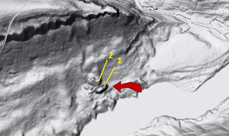
I got tipped off to this feature when a friend posted a shot of the lower boulder (the one with the measurement bar, above) on Facebook, shown below. It’s an impressive image, and gives a sense of the boulder’s scale relative to human observers. The second image below uses a large arrow to show the general perspective of the photo, which also gives a glimpse of the second boulder (2) in the background.
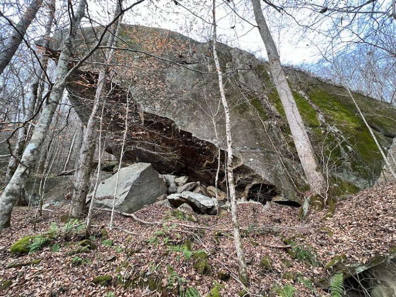
The path carved by the boulders is as wide at the boulders’ long dimension, which suggests (I think) that they slid into place instead of tumbling, without turning much on the way down. The plowed-up path appears to be about 10 ft (3 m) deep, but is entirely re-vegetated with no obvious distinction in vegetation. The additional photos of the boulders below show that they are now just “part of the forest,” so to speak.
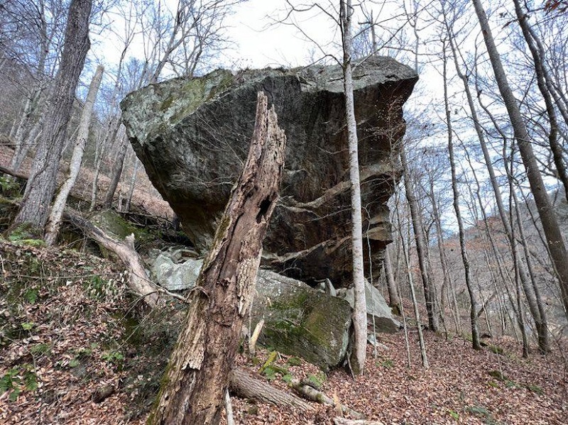
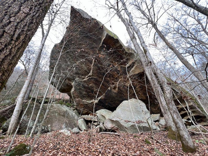
The boulders are Pennsylvanian-aged quartz-rich sandstone (possibly Rockcastle Formation?), so they are physically and chemically very tough and look to be well-preserved. I have not personally been to these boulders, but it’s likely that a geologist could easily establish which sides of the boulders were facing up and out (the old cliff face) prior to detachment and emplacement. Reddish-brown oxidation on the underside of the boulder in the image above might be a clue to this sort of interpretation, but I’m not sure.
The boulders are located along the Big South Fork National River, which carves a steep gorge through the Pennsylvanian-aged geologic section in northern Tennessee and southern Kentucky. The river itself is full of boulders in this area, but most are processed out of the lidar data. The Google Earth image below shows the river in the vicinity of the giant boulders, and is paired with a matching lidar overlay for reference to the tracked boulders.
This “tracked boulder” example is particularly interesting because it provides direct evidence that the boulders traveled overland to their resting place, likely in one big event. Falling, sliding, or tumbling during a major failure are not the only ways boulders might move downhill. Rapid weathering of weak or soluble rocks below the cliff line might allow pieces of the cliff line to be gradually lowered as the underlying bedrock weathers away, causing a former cliff line position to decay into a line of scattered boulders. Boulders might also slowly creep downslope if the underlying soil or rock are sufficiently unstable, particularly during wet climatic patterns or aggressive freeze-thaw cycles. I think (but am not entirely sure) that both of these non-falling processes are either documented or suspected in cases of apparent large boulder movement elsewhere in the world. In this Big South Fork case, however, the physical evidence suggests the boulders failed and slid in an impressive event and plowed a 3 m (10 ft)-deep path down the slope. Knowing that boulders can and do move like this in the Cumberland Plateau landscape is useful to understanding potential hazards and how best to interact with the landscape, particularly from an engineering standpoint.
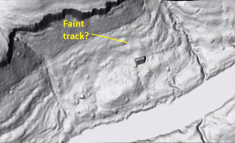
Understanding why more boulder tracks aren’t visible in a region as bouldery as the rugged parts of Appalachia (throughout its provinces–not just sandstone-capped Plateau areas) is another interesting question. Plenty of large boulders are found near the tracked example discussed here, but none show any obvious surficial evidence of their path downhill. One 28 m (~90 ft) long boulder immediately downstream might be argued to show a well-weathered track, but detailed analysis of soil in the possible track relative to surroundings might be necessary to confirm it. I don’t think the lidar-derived imagery alone is convincing enough.
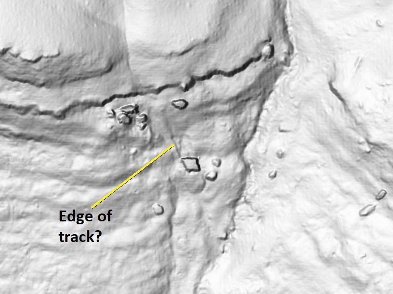
The only other good candidate I have seen in the Cumberland Plateau occurs about 200 km (125 miles) southwest, across the Sequatchie Anticline from Chattanooga, Tennessee. This 20 m (65 ft) boulder, also of Pennsylvanian sandstone, appears to have left a short track, though its point of origin is unclear. A scar shaped like the boulder’s upslope edge may be visible just uphill, suggesting a small amount of travel that occurred after the boulder was separated from the outcrops upslope.
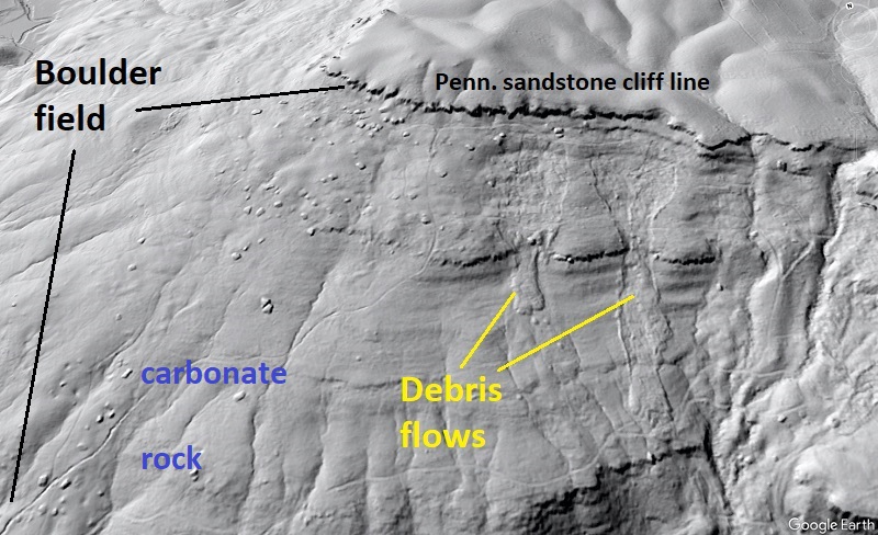
Many Cumberland Plateau slopes are absolutely covered in boulders, but are comparatively gentle (less than 20 degrees) and seem less likely to support rapid and significant boulder travel by slide or rockfall events. The slope shown below is a good example. It is covered with 15 m (50 ft) boulders that suggest association with the cliff line, but just how they ended up so far from the cliff line on a <20 degree slope is another question. Here, dissolution of carbonate rock may indeed play a role, suggesting evolution of the landscape visible in the image represents a very complex interplay of processes. The cool debris flows are an added visual bonus–did they mobilize any boulders?
This post is Cumberland Plateau-focused because the rock types and structure that produce its landscape make visually impressive boulder examples, but the questions raised here apply to the Appalachian Plateau to the north, the Valley and Ridge, and the Blue Ridge and westernmost Piedmont. All of these provinces host many impressively boulder-covered slopes, and seldom do the boulders offer any evidence of when or how they ended up where they are today. Understanding boulder separation from outcrops and downhill movement goes beyond just being interesting–it can improve understanding of how climate history shaped the landscape as well as how dynamic hillslopes can be. As lidar-derived imagery offers a new way to look at boulders on forested slopes, geologists are likely to greatly expand understanding of Appalachian hillslope evolution in coming years.
You May Also Like
Pleistocene Coastal Plain sand dunes and the value of pattern recognition in LiDAR interpretation
Lidar imagery reveals details of debris flow movement in the eastern Blue Ridge Mountains of North Carolina
Low-displacement landslides explain unusual West Virginia landscape features visible in lidar imagery
-
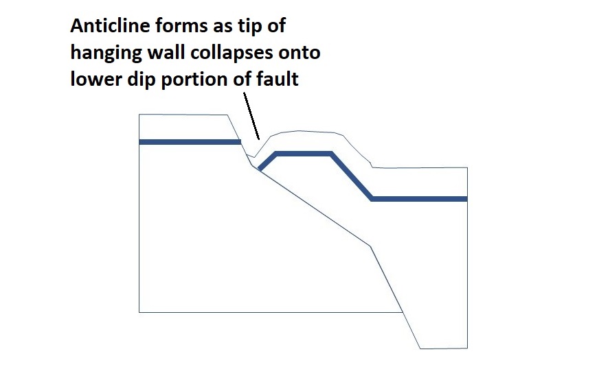
Extensional anticlines along normal faults
Anticlines (convex-up fold structures in rock layers) are often associated with compressional tectonic forces which cause layers to buckle and fold. Anticlines can also develop when extensional forces produce normal faults in a rock mass, provided the steepness (dip) of the normal faults changes with depth. Anticlines that form due to a downward decrease in fault steepness are generally called rollover anticlines, and are a form of fault-bend fold. This post shows a conceptual diagram of this process, some sandbox models containing extensional anticlines, and a real-world examples.
These minor anticlines form when the hanging wall block (the block of layers dropping downwards) must change its shape to match underlying footwall block along which it is sliding.

The “gaps” shown between the dropping hanging wall and the footwall in the sketches above don’t actually form in a model or the real world; I just use them to illustrate the shape mismatch. The upright anticline that forms results from an initial fault propagation fold that forms one antilcine limb, followed by collapse of the edge of the hanging wall to produce the other limb.
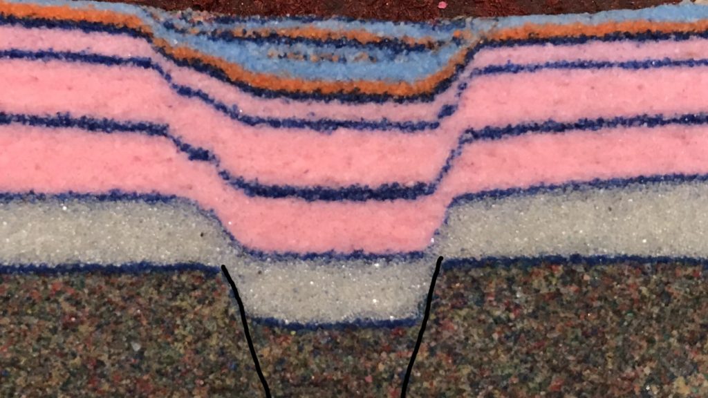
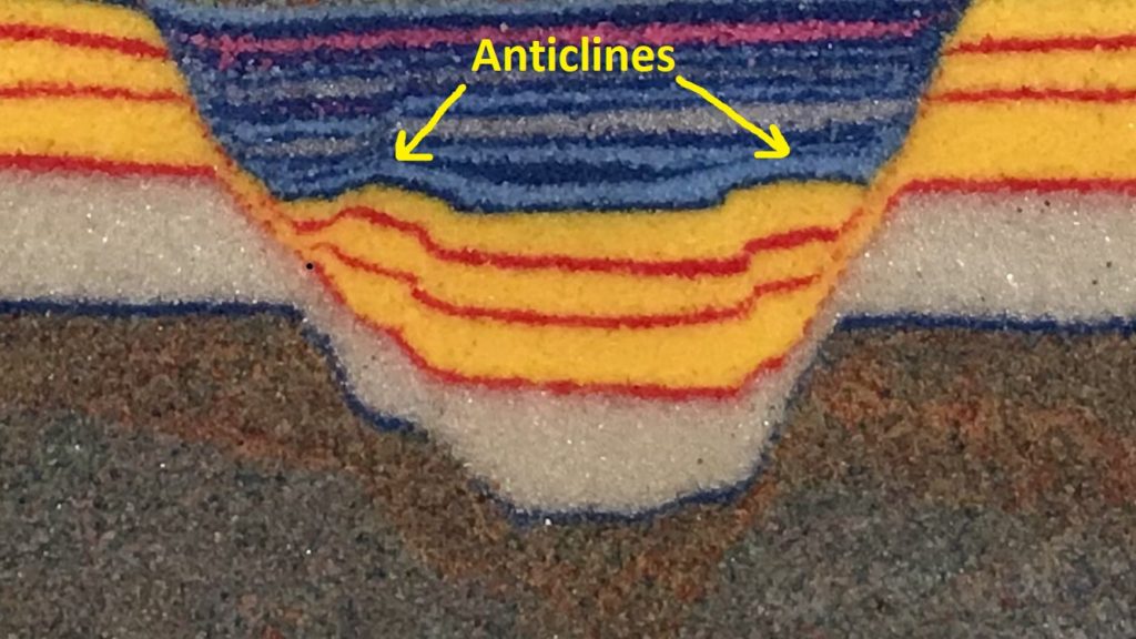
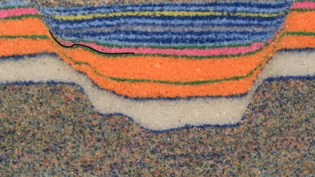
This image corresponds to the first movement phase in the sketches. The image above shows the fault propagation fold stage, where the pink layer bend downwards above the broken gray basement layer at the bottom. If the model had been extended further…
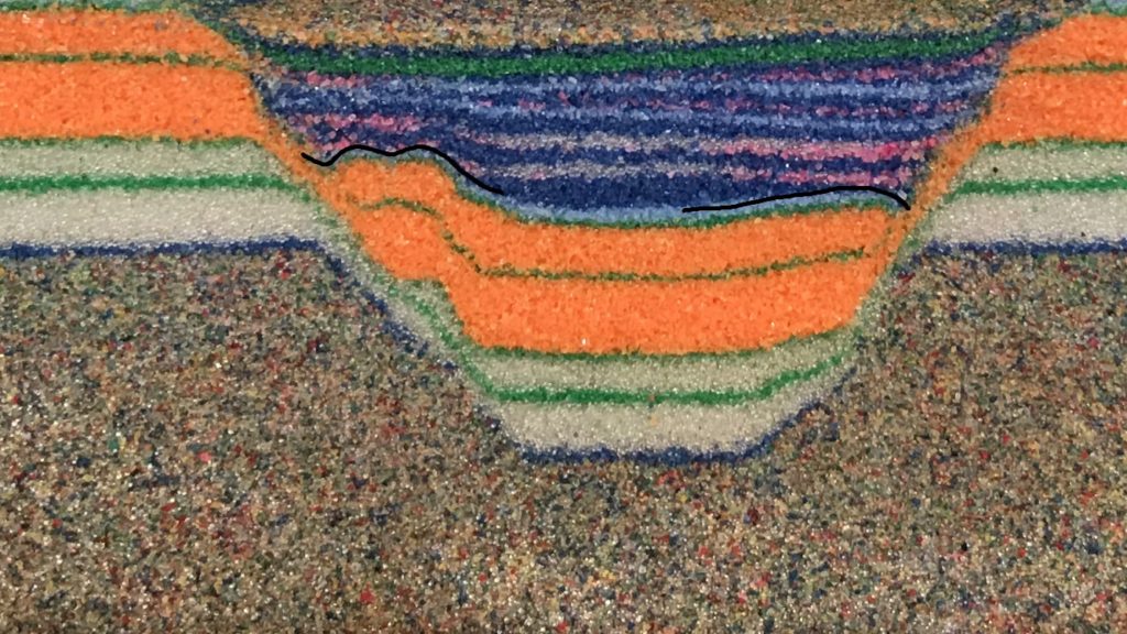
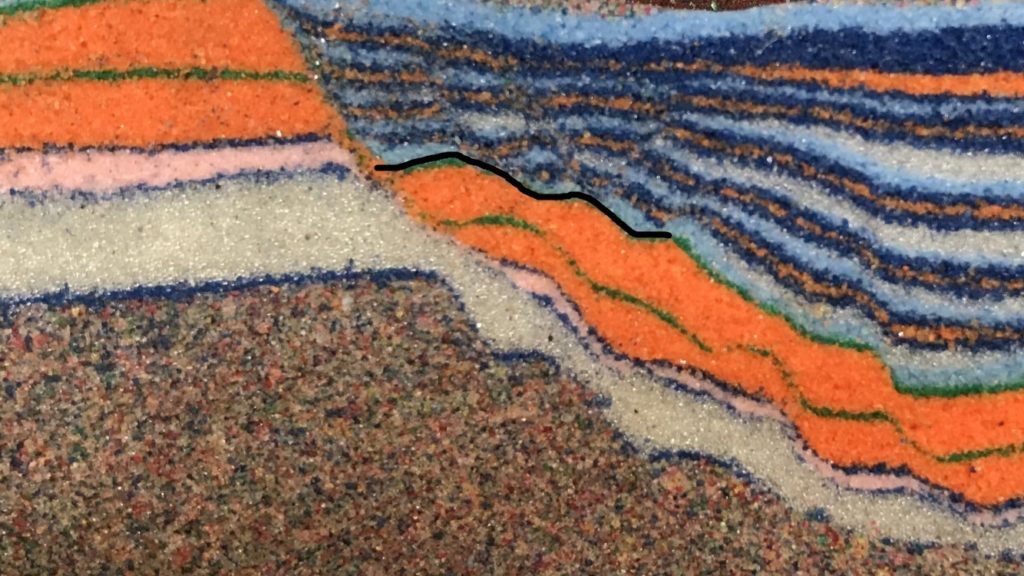
…it would look something like this. The left side of the hanging wall block (the downthrown block in the middle) has formed a closed, convex-up anticline in the orange layers. Compare it to the sketch below, the last phase of the moving image near the top.
Below are a few more examples. In each case, the normal fault dips less steeply in the weak white layer, causing collapse of the overlying hanging wall and forming an anticline.
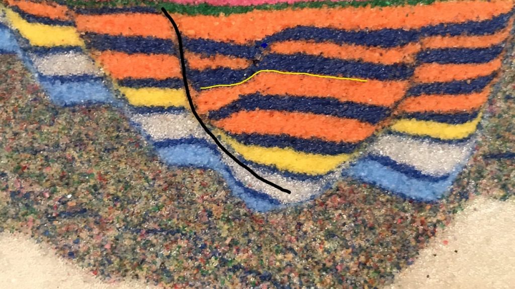
This model is set up a bit differently, so there is no fault propagation fold to make one of the anticline limbs. There is still a downward-flattening normal fault, though (black line), so an asymmetric anticline (the thin yellow line runs along the top of it) formed. Like in all the models, the normal fault became shallower in the weak white layer. 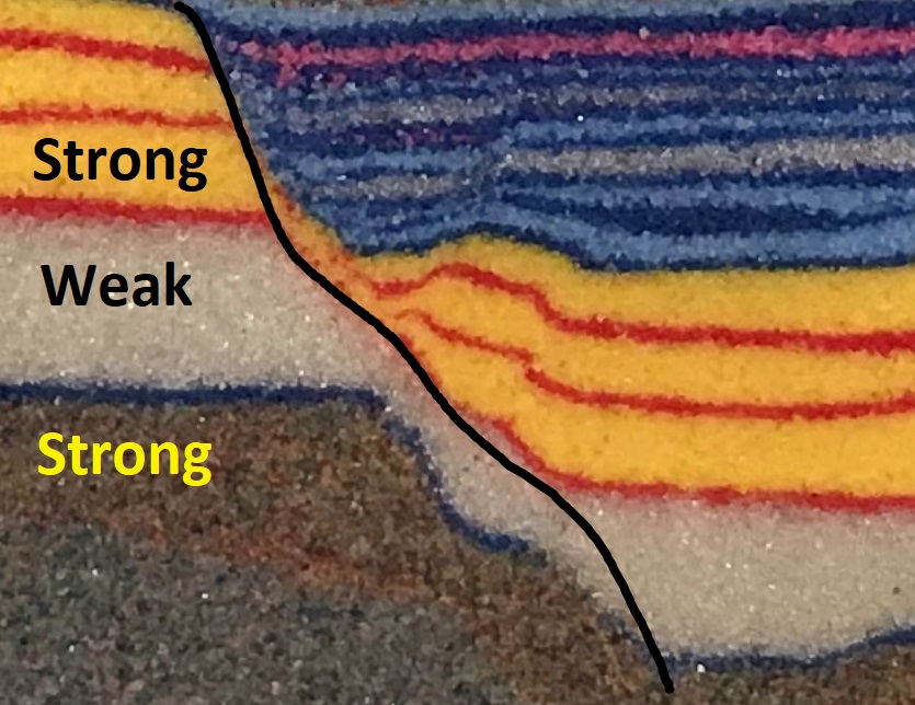
My favorite example…the normal fault (black line) shallows in the weak white layer, closing the anticline. The right limb of the anticline actually has a small reverse fault in it (read about it here. The collapsed left limb of the model anticline above resembles the collapsed limb of the hanging wall in the Jeanne d’Arc basin off of Newfoundland, shown below (image sourced here).
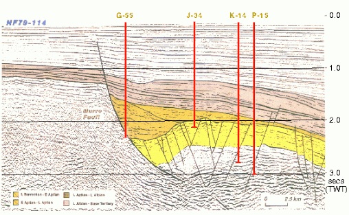
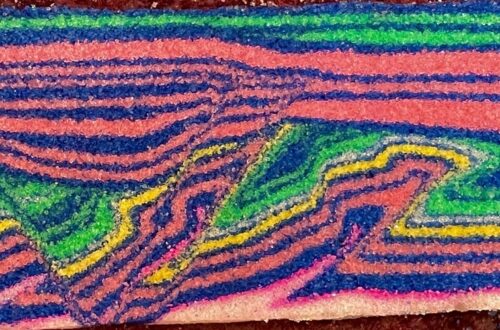
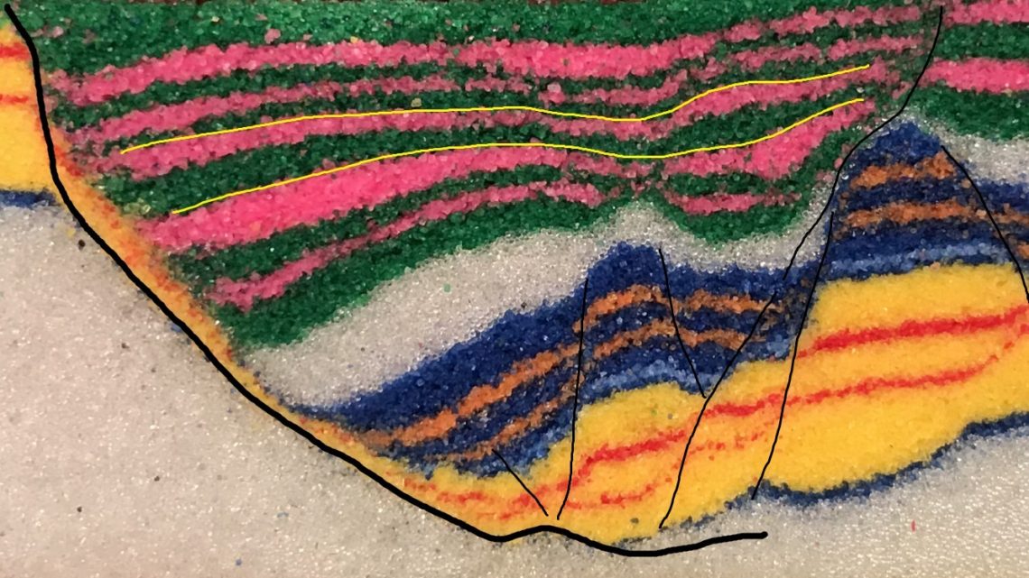
The change in the dip of the main normal fault can be seen here; it produces the rollover folding in the same way that it forms in the models. The next model image uses a slightly different setup, but the same downward flattening of the normal fault is still apparent. Here, another week layer within the hanging wall partially “disconnects” the pink and green layers from everything below, allowing them to form very gentle, broad folds above more intensely faulted layers.
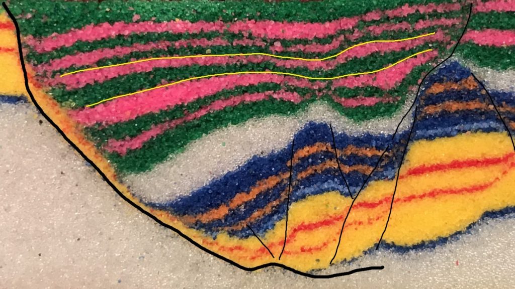
The pink and green layers are nearly faulted, but not quite…the yellow and dark blue sequence below is a different story.